Nucl. Energy, 34, No. 2 Apr., 85-91, 1995.

This Paper was first presented at the BNES seminar "Applications of artificial intelligence in the nuclear industry", London, September 1994.

On-line control of the COMPASS-D tokamak using a neural network

C. G. Windsor+, P. S. Haynes*,D. L. Trotman*, M. E. U. Smith*,T. N. Todd*,M. Valovic*

+ B521, AEA Technology, Harwell, Oxon

UKAEA Fusion, D3, Culham Science Centre, OX14 3DB, UK

Abstract:
Multi-layer perceptron (MLP) networks are particularly appropriate for performing rapid non-linear mopping. In the application discussed in this paper the position and shape of the plasma within the experimental fission research tokamak COMPASS-D at UKAEA`s Culham Laboratory is determined from a series of magnetic sensors placed around the vacuum vessel, close to the plasma boundary. By using a real-time analogue neural network it is possible to achieve control within a sub-millisecond time-scale. In this application the neural network is needed to solve an inverse problem. Numerical codes exist that are able to calculate the signals expected on the magnetic sensors for a given plasma position and profile. The problem is well defined from the solution of the Grad-Shafranov equation. However, no easy analytical formalism exists to reverse the problem to calculate the plasma parameters given the magnetic signals. It is this mapping, from the set of magnetic diagnostic input signals to the parameters of the plasma, that an MLP network can be trained to solve. The training data are some 2000 example plasma equilibria, covering the likely possible configurations of the plasma, solved by numerical methods. The desired aim, to control the plasma boundary position to within a few millimetres, has now been achieved.

1. Introduction

Neural networks are now established as statistical tools that give significant advantages over conventional methods when used in appropriate applications.¹ The artificial networks of a few thousand neurons that can now be built fall far short the human brain, which has about 10¹⁰ neurons and 10¹⁴ connections. They do, however, have the advantage of electronic speeds compared with the brain's much slower chemical processing. The ESPRIT project ANNIE, led by AEA Technology, on industrial applications of neural networks² succeeded in comparing neural networks with the best state of the art conventional methods. Applications considered were defect classification in pattern recognition, robotic collision avoidance and optimization of aircraft crew scheduling. A generic conclusion was that although in many applications neural networks gave no significant improvement in performance, they could dramatically enhance speed. In the classification of weld defect from ultrasonic data, for example (considered within the project), a neural network gave essentially the same performance as a classical adaptive receptive field classifier trained on identical examples, but was fast enough to be able to operate on-line.³

A more fundamental advantage over most conventional methods, however, is the ability of neural networks to perform non-linear mappings of arbitrary complexity. The essence of neural network methods is the single neuron, Fig. 1, which delivers an output that is a non-linear function of the inputs received from other neurons, Each neuron may be considered as a low-level feature detector that seeks out patterns it has been trained to recognize in the input data.A second layer of neurons then takes these low-level features as its input data, and generates the high-level features that are needed for pattern classification or process control. In the example in Fig. 1, the

Fig.1. A single neuron and its mathematical model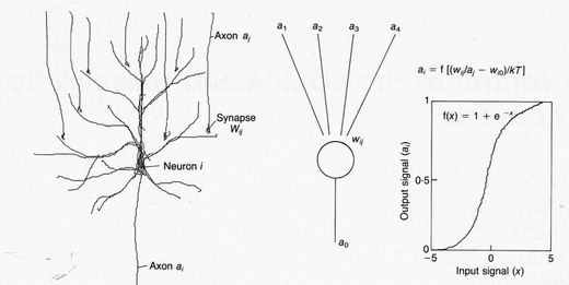

dendrites of the i^th neuron accept signals a_j from the axons of other neurons j. The synapses modify the input signal in a way modelled by the weight w_ij.The output signal aⁱ depends on a sigmoid function f(x) of the weighted sum of inputs less the threshold w_i0, divided by an equivalent thermal energy kT. The inset shows the mathematical form of the sigmoid function simulated by the network hardware. It is the presence of the second set of non-linear elements that has made the three-layer MLP the dominant method in current neural network practice. Its static nature (e.g. in this application it makes no attempt to follow the time dependence of the mapping) may mean, however, that it will be superseded by dynamic recurrent networks. The MLP illustrated in Fig. 2 has the three-layer structure implemented in hardware on COMPASS-D. Neurons in each layer of the MLP are fully connected to neurons in the layers above and below, but not within the same layer or across layers. Its function is to perform a non-linear mapping from the input to the output space. On COMPASS-D at present, 32 input variables, which represent various magnetic diagnostic signals, are mapped into a two-dimensional space that defines the top of the plasma and its elongation x. Because arbitrary amplitudes are possible for the weights the input variables may have all sorts of different magnitudes, units and functions. They may equally be control currents in kilo-amps, or soft X-ray amplitudes. The neural network is able to fuse such diverse data to make its 'decision' just as the human operator is able to assimilate information from the many displays in the control room.

The ANNIE project concluded that neural networks could give dramatic benefits in the speed of operation after training. The training is a good one. Contemporary management recognizes that training is an investment, even if it requires many hours of dedicated effort, both from the teacher (who selects and appropriately presents the material to be learnt) and from the student. To train a neural network, training data must be collected or simulated and transformed into such a form that the network is not swamped with or denied information. With each training example (point on the input mapping), must go the corresponding target (point on the output mapping). This may be a classification, such as a 'crack' defect, or a parameter, such as the elongation of a plasma. During training the examples are repeatedly presented to the network together with the targets, and the weights of the network adjusted iteratively until the match between the network outputs and the targets is as good as possible. This is a relatively long process, a few hours on a PC for the COMPASS-D network.

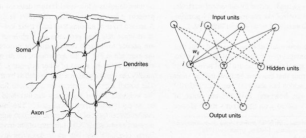
Fig.2 Multilayer perceptron neural network compared with a portion of cortex.

Outside the research environment, however, it is a one-off task, and does not have to be repeated unless the training data or targets are changed. The trained network, like the trained human, must be considered a valuable asset to any business. The network trained to classify defects from ultrasonic signals, for example, can truly be considered to encapsulate at least some aspects of the experience of a trained inspector. The trained network for tokamak control encapsulates some four box-files of 'shots', each detailing the shape of the plasma for particular sets of diagnostic inputs.

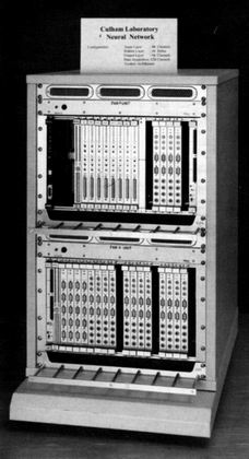
Fig. 3. The hardware implementation of an MLP neural network in use on the COMPASS-D tokamak at UKAEA Culham Laboratory

Once the long training stage is complete, operation of the network in its 'feed forward' mode - where inputs are presented to the network and an output is calculated - can be very fast. The phrase 'parallel distributed processing' describes the key to the speed of operation. Each neuron in any one layer can operate independently from any other in evaluating its output sum. By using independent analogue or digital processors, the necessary calculations can be performed simultaneously in a time determined by the band width of the analogue circuits or the cycle time of the processors. The analogue circuits used in the UKAEA tokamak control application at Culham, shown in Fig. 3, have a band width of 100 kHz and are able to evaluate their outputs in ~10 ms. Such a result is not currently achievable by any conventional digital method. The three types of card needed for a 32 normalized input, 15 hidden unit, 2 output network now sit within a single crate.

Most of the applications of neural networks remain implemented as software simulations. The Applied Neuro-computing centre at AEA Technology, Harwell, has developed several such applications to the stage of commercial software products.⁴ The Centre is now able to undertake consultancy and development contracts involving application of neural networks to a variety of problems, including pattern recognition, elastic matching, process control, sound assessment and data mining.

2. The problem of tokamak control

Fusion power offers environmental and safety advantages over any known alternative power source.⁵ The world is cooperating in the design of a demonstration fusion reactor, 'ITER', with a sustained burning plasma, to begin operating around 2010. Technical problems remain, such as how to control the position and shape of the plasma boundary within the ITER containment vessel to within a centimetre or so. Facilities such as the COMPASS-D tokamak at Culham are test beds on which to confirm the feasibility of novel control methods which might meet this specification.

Fig. 4. The COMPASS-D tokamak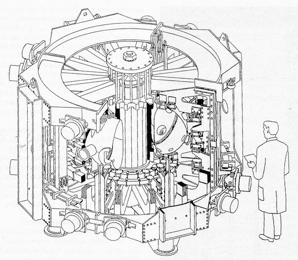

Figure 4 shows COMPASS-D and Fig. 5 illustrates its neural network control circuit. The plasma lies in a toroidal vacuum vessel with a D-shaped cross section. Powerful currents around the centre column and torus act as the primary coil of a transformer whose secondary coitis the plasma itself. Within the vacuum vessel, isotopes of hydrogen at low pressure are ionized and heated to form the plasma. One key to obtaining plasmas with the necessary densities, temperatures and energy confinement times is the shaping and positional control of the plasma. COMPASS-D has a series of special coils and fast-amplifier circuits for this purpose. These are programmed to elongate the plasma from its initial circular shape to a complex shape lying in a precisely calculated position within the vessel.

Various diagnostic systems are used to determine the plasma shape and positional parameters at any instant. Some 32 magnetic coils selected from hundreds placed around the vessel measure the magnetic fields and fluxes produced by the plasma. The outputs from the coils are used as inputs to the present system. It is hoped to use in the future additional inputs from soft X-ray emission profiles. The existing conventional control system uses linear combinations of selected inputs to drive simple feedback loops in the radial and vertical directions. The linear nature of these methods, however, means that they cannot be expected to work accurately over the wide range of plasma shapes encountered,even in a single shot.

Fig.5. The neural network control system implemented on the COMPASS-D tokamak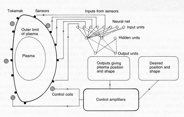

In contrast, the neural network is able to predict selected plasma parameters precisely over the whole range of shapes within the training database.⁶ The training database has been slowly built up by choosing values for the control and shaping currents and for the plasma current density functions. These are entered into a numerical solution of the Grad-Shafranov equation to find the corresponding equilibrium plasma shape. Many of these simulated example shots have been selected randomly from configurations that give rise to possible plasma equilibria. Others have been designed as small random perturbations from actual plasma shapes occurring at selected times throughout the shot. A database of over 2000 shots is now available, defining the detailed mapping between the magnetic inputs and the plasma shape parameters.

3. Training the neural network

The use of standard back-propagation and conjugate gradient descent methods¹ makes this a straightforward task. There are many variables to optimize but a well-defined quality function to minimize - the least squares differences between the targets and the network outputs. A key variable is the number of hidden units. This defines the total number of adjustable parameters in the network and so the degree of detail by which the mapping can be described. Figure 6 shows the learning curve for networks with different numbers of hidden units. The residual fit to the training data continually reduces with iteration number and with hidden unit number. The test performance shown in Fig. 7, however, shows a minimum residual at around 15 hidden units, which was therefore chosen for the size finally used in the hardware. The larger networks fitted the training data better but 'over-fitted' and failed to generalize accurately when presented with test data.

Fig. 6. Learning curve for 15 input, 3 output networks

A second key parameter is the number of outputs. Figure 8 shows the test performance as a function of the number of outputs, showing, as expected, a steady degradation with increasing number of outputs. The chosen network had just two outputs while a network of eight outputs gives only one third the accuracy. An eight output network is capable of giving a good parametric description of the plasma boundary and will shortly be used to drive a visual display. The principal output desired by the COMPASS-D operating team in the near-term was the height of the upper plasma boundary at the radial position of a reciprocating Langmuir probe, which had recently been installed. Figure 9 shows the training and test performance for the network output compared with the actual boundary height when using the same set of trained weights and input variables. The root mean square difference in training is 25 mm and in test is just 30 mm.

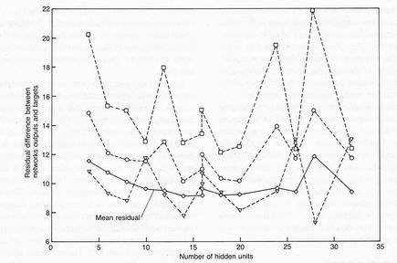
Fig. 7.Test performance using example shots not used in training. Dashed lines: individual outputs

The weights of the trained software network can be down-loaded directly to the VME bus controlling the hardware network. The network also receives an input giving the plasma current, which is used to normalize electronically the network inputs to the constant plasma current used in the training data. The performance of the network was tested by a simulation program in which both the final outputs, and the intermediate inputs and outputs to each sigmoid, could be compared with a simulation based on the recorded input variables as a function of time. The hardware reproduces the standard sigmoid neural transfer function

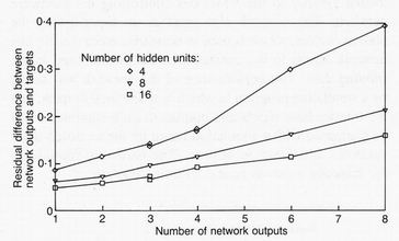
Fig. 8.Test performance as a function of the number of outputs and number of hidden units

f(x) = b[l/{l + exp(-ax + g)}]

and simulation is able to take into account, if required, the measured small deviations of the sigmoid amplitude b and exponent a from their design values, and the measured offsets to each sigmoid. Figure 9 shows an example of the actual and simulated output representing the upper plasma boundary height at the radius of the reciprocating probe.

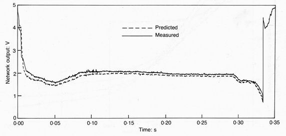
Fig. 9.Simulation of the hardware neural network
3. On-line control of the plasma boundary

When in operation, the `plasma top' output is wired to replace the existing linear height estimator. Its value is compared with a programmed height waveform for the shot and the difference is fed to a circuit that drives the fast amplifier, which controls the vertical position. Figure 10 shows the probe height desired output (Z_ref) compared with the network output (Z_probe). The programmed vertical position was given a 20mm ramped change at 140 ms. The network output is seen to reproduce this change precisely. The sharpness of the edges of the ramp demonstrates the sub-millisecond response time of the network. The true performance of the network can be assessed from television pictures of the visible light emitted by the plasma. The images in Fig. 11 show the top of the plasma directly and readily show the shift at around 140 ms. In a second shot the plasma elongation was programmed to change while the upper plasma boundary was maintained at a constant position. Other shots have demonstrated the increase of elongation of the plasma under programmed control.

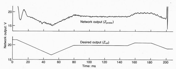
Fig. 10.The network output of plasma height compared with desired profile

4. Conclusions

This project shows that sub-millisecond control is possible using a hard-wired neural network even for this most complex of problems. The MLP network is shown to be able to perform the required mapping of 32 magnetic inputs to plasma height with an acceptable error of around 3mm. The hardware implementation of the chosen network was able to accommodate the 15 hidden units network suggested by software optimization. It has proved straightforward to operate and is easily loaded with new network configurations and trained networks, It should be possible to use the hardware developed by the Culham team to implement similar control schemes.

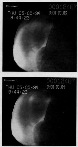
Fig. 11.Television pictures of the visible light emitted from the plasma before and after the programmed rise in the plasma upper boundary: images ageraged between 140-160 ms (top) and 180-200ms.
6. References

1.. RUMELHART D. E. et al.Learning internal representions by error propagation, Parallel distributed processing. MIT Press, Cambridge. MA, 1986.

2. CROALL. I. F. and MASON J. P. (eds) Industrial applications of neural networks. Springer Verlag. 1991.

3. WINDSOR C. G. et al. The classification of defects from ultrasonic images: a neural network approach. Brit. J. NDT; 1993, 5, 15-22.

4. MASON I. P. et al. A novel algorithm for chromatogram matching in qualitative analysis. J. High Res. Chromatag., 1992, 15. 539-547,

5. O'BRIAN M. and ROBINSON D. Setting the course for a commercial power plant, ATOM, 1994, 434, 32-35.

6. BISHOP C M. et al. Hardware implementation of a neural network to control plasma position in COMPASS-D. Fusion Technol., 1993, 997-1001.