Euratom-UKAEA Fusion Association, Culham Science Centre, Abingdon, OX14 3DB, UK

Accepted for publication 6/8/2008

Abstract

A prediction has been made of the Charpy ductile-brittle transition temperature at high irradiation levels from a dataset of 459 low-activation ferritic/martensitic steels. It follows a similar study of the yield stress of some 1811 similar alloys (Windsor et al, Modelling Simul. Mater. Sci. Eng. 16 (2008) 025005). Neural networks have previously been used by Cottrell et al (Journal of Nuclear Materials 367-370, 2007, 603-609) to model the Charpy ductile-brittle transition temperature of these alloys. The same dataset has been used in this study, but has been divided into a training set containing the majority of the dataset with low irradiation levels, and a test set which contains just those alloys which have been irradiated above a given level. For example, some 7.2% of the dataset was irradiated above 20 dpa. Good predictions were made using two different codes and methods. As with the yield stress prediction, the target-driven components method, where linear combinations of the atomic inputs are chosen to reduce the test residual, achieved the best results.

1. Introduction

The Charpy test measures the toughness of a material: that is, its ability to absorb energy during fracture [3]. The experimental work used in this paper used sub-sized specimens made by machining 3.3x3.3 mm² rods with a 45^o angle notch in the centre. A heavy hammer is swung onto the specimen and the energy absorbed during fracture is measured by recording how far the hammer rises beyond the specimen. This measurement alone is somewhat qualitative, but more quantitative information can be obtained by recording the results as a function of specimen temperature. Most ferritic alloys undergo a 'ductile to brittle' transition. At high temperatures the fracture is ductile with relatively high energy absorption. As the specimen temperature is reduced there is a transition to brittle fracture, with much lower energy absorption. The fracture surface also changes from a 'torn' ductile fracture surface to a rough surface showing inter-granular separation. The change with temperature is generally quite sharp and from the central temperature of the distribution a ductile to brittle transition temperature may be reliably inferred. This work is concerned with the ductile-brittle transition temperature shift (DDBTT) as a function of irradiation. An example of the Charpy curve and the effects of radiation are shown in figure 1 [4]. The un-irradiated alloys are assigned a zero shift, and the change in temperature is measured as a function of irradiation level.

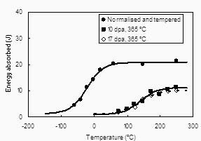
Figure 1: Charpy curves for half-size specimens of 12Cr-1MoVW steel before and after irradiation to 10 and 17 dpa at 365C in the Fast Flux Test Facility [4].

It is known that specimen size affects the ductile-brittle transition temperature in Charpy impact testing [5], and there is some evidence that sub-sized Charpy tests provide non-conservative estimates of embrittlement [6]. However since this paper deals only with sub-sized specimens we expect our predictions to be internally consistent.

The importance of the Charpy toughness test is evident from its use in the British Energy R6 validated procedure for assessing the integrity of structures containing defects against failure under operational or fault loads [7]. Material toughness may be analysed using the Beremin model which is able to express the fracture probability in terms of the Weibull parameters fitted to the Charpy data [8].

The database used in this work is concerned with irradiated low-activation martensitic steels, and was compiled from the literature by Yamamoto et al [9]. In all some 459 specimens were included in the database with irradiation levels up to the fusion reactor relevant range of order 100 dpa (although the particle energies are lower than those for fusion irradiation). Figure 2 shows the ductile-brittle shift with irradiation as a function of irradiation level.

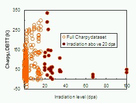
Figure 2: The change in ductile to brittle transition temperature in degrees Kelvin with irradiation level measured as a function of irradiation level in displacements per atom (dpa). The full dataset has been divided into training data at low irradiation levels (open circles) and test data at irradiation levels above 20 dpa (closed circles).

The figure shows many data at low irradiation levels, with some 7.2% of the database at levels greater than 20 dpa. There is an appreciable spread (over 250 degrees K) in the Charpy shift at any given irradiation level, partly because of the varying compositions of the individual steels, and partly because of the varying normalising temperature, normalising time, tempering temperature and tempering time which differ for the different steels at the same irradiation level. It will be shown later in figure 3 that the inclusion of these variables leads to a much reduced spread in the fit to the training data of around 50 K. On an expanded irradiation level scale it is seen that all the Charpy shifts for un-irradiated specimens are indeed zero. However for irradiation levels around 5 dpa, the measured shift can and does have positive or negative values. It is seen that the trend of the average shift rises up to around 25 dpa, as illustrated in figure 1, then falls because of irradiation softening [9].

A fusion reactor needs structural steels that will be able to withstand irradiation levels in the range 20 to 90 dpa, but obtaining high-dose data is expensive and time-consuming. As figure 2 suggests, there is at present only limited data in this range. An objective of this work is to determine how well Charpy measurements taken at lower irradiation levels may be used to predict properties in the reactor-relevant range. It is important to note that there are likely errors in both the Charpy shift and the irradiation dose axes of these graphs. An estimate of the Charpy shift error can be made from the work of Mueller et al [10] as around +/- 20 K. The irradiation dose error arises from the difficulties of integrating the reactor or accelerator power over an irradiation which may last many months or years. It is likely to be several percent. A further relevant source of errors is in the measurement of alloy chemical compositions, which are also subject to an uncertainty of several percent. In some additional cases these were also incompletely described in the database and had to be estimated from other sources in the literature. Where the missing information was related to impurities, which are inevitably present (i.e. Cu, O), the composition was set to be equal to the average of the available data.

2. Performance assessment: the test residual

A problem, common with all highly-flexible least-squares fitting procedures, is that in order to test the fit, the dataset must be divided into subsets of "training" and "test" data, where none of the test data has been included in the training process. This paper will use the root mean squared least squares test residual R_test defined as the square root of the summed squared difference between the network targets T_i and calculated network outputs O_i, divided by the number of test examples N_test

R_test={[ S_test ( T_i - O_i)]/N_test}^1/2 .....(1)

where the summation i includes only the test examples chosen from the dataset. Here T_i are the network targets, essentially the experimentally-obtained values of the DDBTT for each example alloy in the dataset. O_i are the outputs of the trained neural network. With the Charpy ductile-brittle transition temperature shift (DDBTT) as target, the residual has the units of degrees K and is essentially the root mean square deviation between actual and predicted shifts. The main neural networks code used is an adapted version of the MAGEOM code written by Colin Roach and Paul Haynes under the direction of Chris Bishop [11]. It is able to perform the target-driven components method described in section 3. It does not contain any error determination in the ways used in reference [2]. To supplement this code, its main conclusions were confirmed with the "BIGBACK" code written by David MacKay [12]. This was run using the interface code "Model Manager" [13]. It includes a full Bayesian error treatment. In particular it is able to lower the weightings of irrelevant variables automatically.

If all the dataset had been used for training as described in Cottrell et al [2] then, as considered by them, the optimal number of hidden units is between 4 and 6.

3. Neural networks used in a predictive mode,

The long term objective of this study is to predict the change in Charpy shift under the conditions of a fusion reactor, say for irradiation levels above 40 dpa. There are at present very few data in this region and the present study seeks to remedy this by asking whether predictions from lower irradiation levels might make a useful prediction at fusion reactor levels, as well as using the modelling technique to provide insight into radiation embrittlement mechanisms. While the accuracy of such predictions is unlikely to be good enough for structural safety evaluation, it may well be sufficient to say whether today's alloys, with measurements at only relatively low irradiation levels, may be useful for reactor applications, or whether new alloy development is essential. As more data become available at high irradiation levels we expect our model to be more precise. The neural network predictions, used for this dataset by Cottrell et al [2] made no attempt to address this problem. They used the conventional approach, dividing the whole dataset into equal randomised training and test datasets, and optimising the network test performance. A different strategy is used here and was used in our earlier work on yield stress under irradiation [1]. Here the data at low irradiation levels is used as training data, and the data at high irradiation levels as test data. There is therefore no uncertainty in test performance arising from differing choices of training data. The irradiation level of 20 dpa has been chosen here since it leaves a reasonable proportion (7.2%) of the dataset for testing. It will be shown that, at this level, the network is indeed a good predictor of performance, and that such networks optimised for test at high irradiation level can be quite different for those optimised for performance over the whole dataset.

The dataset contained a single target parameter, the change in ductile/brittle transition temperature, and 26 input variables. The input variables may be divided into 7 non-atomic inputs

i) normalising temperature, range 273-1473 K
ii) normalising time, range 0-2 hours
iii) tempering temperature, range 273-1053 K
iv) tempering time, range 0-780 hours
v) irradiation temperature, range 333-823 K
vi) irradiation dose, range 0-100 dpa

The remaining 19 input variables detail the atomic fractions of selected elements. These include the elements C, Cr, W, Mo, Ta, V, Si, Mn, N, Al, B, Co, Cu, Nb, Ni, P, S, Ti and Zr. The ranges of some of these atomic fractions are very small.

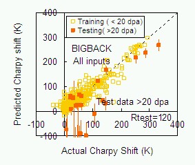
Figure 3: The calculated value of the shift in Charpy transition temperature compared to its actual value for test data having irradiation levels greater than 20 dpa. The calculations used the BIGBACK code including all the available input variables. Hidden unit numbers ran from 1 to 20 and there were 5 seed values at each stage. The run number is 889, and the test residual is 120.0 K. The best individual result corresponded to 3 hidden units.

Figure 3 shows an example of results from the BIGBACK code, including all the inputs detailed above, when training is carried out for the examples with irradiation levels below 20 dpa and testing is for those examples at greater irradiations. This is not the normal usage of BIGBACK which might conventionally divide the dataset into a 50% training dataset and 50% test dataset. It rather considers how it might best use the training data available to "extrapolate" into the high irradiation range not covered by the training data. It is seen that the open squares representing the training data performance fall reasonably close to the dashed line representing perfect performance. The closed squares representing test data with errors are more scattered although do give a useful predictive accuracy considering that some points are highly extrapolated beyond the training data. Note that the limited size of the total dataset meant that no "validation dataset" was used so that operations like the optimisation of the hidden units were performed on the test dataset.

Using the test data above and for a particular irradiation level, it is easy to see which of the non-atomic "fixed" inputs is most significant, by first including all fixed inputs and then removing one of the inputs and noting the new residual. Such results are shown in figure 4. The left-hand column (light) is when all fixed inputs are included. The other columns (dark) have the input noted omitted from the network. If the data >20 dpa form the test data the prediction accuracy is generally similar or higher, showing that the variable was helpful. However the irradiation temperature input variable is not helpful with a residual less than when the variable was included.

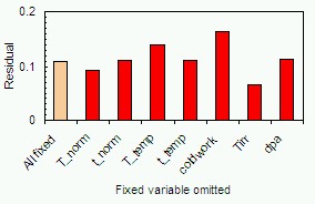
Figure 4: The test data residual when the change in ductile to brittle transition temperature is evaluated from a 5 hidden unit neural network including all the fixed non-atomic inputs "All fixed", (light) and with the other non-atomic variables detailed omitted (dark). This is done for test data at irradiation levels above 20. It is seen that omitting the irradiation temperature input Tirr gives a significantly lower residual.

Turning to the atomic fraction input variables the most relevant variables may be considered by the forward sequential selection of features method [14]. Each atomic fraction variable is added in turn to a network already containing the 5 or 6 fixed inputs depending on whether the irradiation temperature variable is included. Such results are shown in figure 5 for test irradiations > 20 dpa in the absence of the irradiation temperature input. The most helpful atomic inputs to add to the network are those first in the list: C, N, Co and V. A few are above the dashed line and so are not helpful to add at this stage. This result can change later when other atomic inputs have been added.

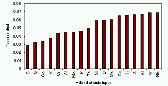
Figure 5: The test data residual when all the potential atomic inputs are added to the fixed variables. The original residual when only the fixed inputs are added is shown by the dashed line. Almost all inputs are helpful. Carbon, Nitrogen, Cobalt and Vanadium are the most helpful at this stage and define the order for the determination of linear combinations.

Following the forward selection of features, the atomic variable whose addition gives the lowest test residual is chosen to be included alongside the fixed variables in the next stage. All the remaining atomic variables are then added in turn to the current network and again the atomic input giving the lowest test residual is included in the following stage. The process is repeated until the addition of further atomic variables fails to cause any reduction in the residual.

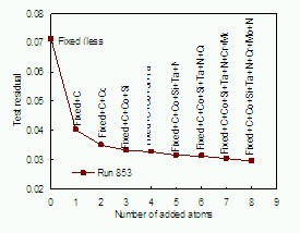
Figure 6: The test data residual during the forward selection of features process. Those atomic inputs are added which lead to the largest reduction of the test residual. The process is continued until there is no further reduction in the residual. This run is for 13 hidden units, with test irradiation levels above 20 dpa, the irradiation temperature input excluded. There were 800 iterations and the results are the best 10 out of 20 runs.

Figure 6 shows this process during the addition of the atomic inputs for C, Co, Si, Ta, N, Cr, Mo and Ni. All these inputs cause a successive reduction in the test residual. However at the final stage, no other atomic input causes a reduction in the test residual.

An important variable is the number of hidden units. In general the residual obtained will show a minimum as a function of hidden unit number. If the number of hidden units is too low the network will have insufficient adjustable variables to fit even the training data. However if the number of hidden units is too high the details of the training data may be "over fitted" to a high accuracy but at the expense of the fit to the test data. The optimal hidden unit number may be estimated by repeating the whole forward selection process as a function of hidden unit number as in figure 7.

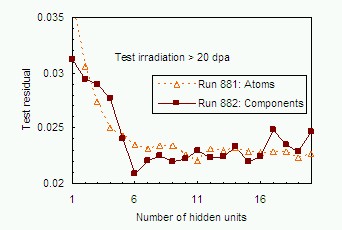
Figure 7: Open triangles show the test data residual at the end of the forward selection of features process as a function of the hidden unit number. The minimum exists at 11 hidden units but is very shallow. The closed squares, to be discussed later correspond to the target driven components method for the same data.

4. The target-driven components method for dimensionality reduction

This method was described in [1]. It seeks to promote the ideal of dimensionality reduction by combining existing atomic inputs A_j into new inputs, X_m, composed of linear combinations of existing atomic inputs.

X_m= S_j P_j,m.A_j ....(2)

where P_j,m are coefficients describing the contribution of atom j to linear combination m. Many of the coefficients P_j,m may turn out to be zero as we expect only those elements relevant to the particular mechanism to contribute to the composite vector.

There will in general be several such mechanisms m for improving the yield stress, and so for improving agreement with the target. Each mechanism will depend on different linear combinations P_j,m of atomic concentrations. One may seek to evaluate in turn several such sets of combinations appropriate for different mechanisms m for increasing the target yield stress.

The method used to derive the coefficients P_j,m in equation 2 begins as in the forward sequential selection of features method, by finding that single chemical element, say C, whose addition to the network together with the fixed variables gives the greatest reduction in the test residual. At the same time all the potential atomic inputs are ordered according to the reduction in residual obtained when they are added to the network as in figure 5.

The method is continued by considering, along with the most salient atomic input (in this case carbon) and the fixed inputs, the possible inclusion of all other remaining atomic variables. These are taken in the order of saliency so that nitrogen is taken first. The next step is to form a linear combination of the inputs from the most salient atomic variable C with those from the second most important N and to observe the trend of the test residual, as the fraction of the second atom is increased. The new variable is

X₁ = (1-f) A_C + fA_N ...(3)

where f is varied from 0 to 1 and A_C and A_N are the individual atomic inputs. Examples of such curves are given in figure 8.

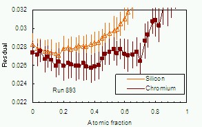
Figure 8: The test data residual when new linear combination inputs are used between the inputs. The light triangles show the effect of adding a given fraction of the Silicon atomic input to the existing best component. The dark squares show the effect of adding the Chromium input to the previous best result obtained. The vertical lines indicate the standard deviations contributing to the average.

This process is continued until the inclusion of extra atomic components gives no further reduction in the residual. This is illustrated by the closed squares in figure 9. The steady reduction in the residual as more single atomic input variables are added is seen for 4 cycles. The atoms added to the combination are N, Co, V and Cr. The process continues until all atoms have been included in the linear combination and the best combination identified. After this point the inclusion of further atomic component inputs gives no further reduction in the residual. The inclusion of many atoms fails to reduce the residual.

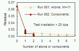
Figure 9: The test data residual when linear combinations of atomic inputs are constructed compared with when single atomic inputs are added. It is seen that the combination inputs give lower residuals than the atomic inputs. The results are for test data at irradiation levels >20 dpa, and with networks with number of hidden units (shown as nh) giving the lowest residual.

The next step is then to consider the addition of a further component. Again the remaining single atomic inputs are added to the fixed inputs and the first combination input. If a reduction in the test residual is found the atomic input giving the greatest reduction in the residual is chosen as the primary component. Linear combinations of this atomic input with others are then made as in the case of the first component. If significant reductions in the test residual are found then these atomic inputs are added to the component. The process of adding component inputs continues until the addition of further atomic inputs causes no further reduction in the residual. The improvement over single atomic inputs is shown in Figure 9.

This process may be repeated for any number of hidden units and the best performance noted. The closed squares and solid line shown earlier in Figure 7 shows the hidden unit dependence for component inputs compared for single atom inputs. The generally lower minimum residuals shown by the target driven component method is clearly shown.

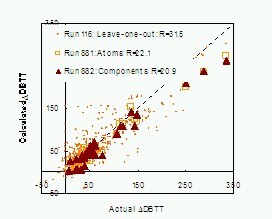
Figure 10: The calculated value of the shift in Charpy transition temperature compared to its actual value. All results are for test results >20 dpa. All exclude the irradiation temperature input, and are for 10 hidden units, 800 iterations and include the best 10 results from 20 runs. The open circles are an example of fitting to all the data using the leave-one-out method. The open squares are for the added atom method, the closed triangles for the target driven components method.

5. The prediction accuracy: scatter plots for various predictions

Figure 10 shows the conventional scatter plot of the predicted Charpy transition shift against the calculated shift for several different calculations and for test data above different irradiation levels. The small faint circles are for a leave-one-out analysis of the whole dataset, and are presented to give an indication of the fitting accuracy when all the data are included in training. The dark triangles are for test data above 20 dpa, and give the minimum residual achieved within a hidden units scan using the target-driven components method. The open squares are the best achieved using added atoms.

The result, clear from figure 10, that the target-driven component method can produce excellent results was confirmed by running BIGBACK with inputs including both the fixed inputs and the linear combinations of atomic inputs derived from the MAGEOM runs. An example of the best results achieved by this method is shown in figure 11. Here the test data are for irradiations > 20 dpa. Interestingly the best results were obtained including the T_irr input but excluding the dpa irradiation level input. The best residual is seen to be 24.0 K, appreciably less than that in the run shown in figure 2 which included all inputs and gave the residual 120.0 K. It is just slightly larger than the value 20.9 K given by the best target-driven component run.

Mode	Atoms	Comp. #1	Comp #2	Comment
Residual	22.1	24.6	20.9	-
Si	-	0.030	-	To deoxidise: Weakens by grain boundary segregation
Ni	-	-	-	Added with Cr, Mo, W as strong carbide formers
Mn	-	-	-	Carbide former: removes weakening FeS
V	7	0.123	-	Scavenges O and forms hardening precipitates
Cr	4	0.800	-	Hard carbide precipitates
Mo	-	-	-	Promotes hard carbide precipitates
W	-	-	0.325	Promotes hard carbide precipitates
C	1	0.028	-	Forms carbide precipitates
B	-	-	0.143	Added to steels to increase hardenability
P	-	-	-	Increases strength and hardness: decreases ductility
S	-	-	-	Decreases ductility and notch impact toughness
Al	3	-	0.337	-
Co	2	0.019	-	Activates under irradiation
Ti	-	-	0.194	-
N	5	-	-	-
Nb	6	-	-	-

Table 1: The first column shows atoms contributing to the best predictions. The second column shows for added single atoms the order of atoms taken in run 881. The third and fourth columns show the components achieved during the target-driven components method for the first and second component. The last column indicates the metallurgical implications.

6. Metallurgical implications

Consider the case shown in the scatter plot of figure 10. Table 1 shows in numerical order the contributing atomic inputs. Generally there are up to around 7 atomic inputs which contribute. The most important in almost every case is carbon (C), the chief carbide former. Chromium (Cr) frequently occurs as a former of carbide precipitates. Silicon (Si) occurs as a common deoxidant. Other atomic inputs occur only sporadically and their occurrence may not be statistically significant. In many case the target-driven components method produces similar contributing atoms. For example run 882, which resembles run 431, generates the following target-driven components: [0.028C, 0.019Co, 0.123V, 0.030Si, 0.800Cr] and [0.143B, 0.194Ti, 0.337Al, 0.325W].

7. Conclusions

Good performance has been achieved in predicting the Charpy ductile-brittle transition temperature above a particular irradiation level (say >20 dpa) from a 459 alloy database trained on data below this level.

The irradiation temperature proved a critical input parameter. Better test performance was achieved when this input variable was excluded, although the training performance was worse.

The best results were obtained using the target-driven components method, where linear combinations of the atomic inputs are chosen which achieve a minimal test residual.

Both the MAGEOM and BIGBACK neural network codes gave good results for the prediction of high irradiation level properties.

Acknowledgements

This work was supported by the United Kingdom Engineering and Sciences Research Council and the European Communities under the contract of Association between UKAEA and EURATOM. The views and opinions expressed herein do not necessarily reflect those of the European Commission.

References

[1] Windsor C G, Cottrell G A and Kemp R, Prediction of yield stress in highly irradiated ferritic steels, Modelling Simul. Mater. Sci. Eng. 16 (2008) 025005

[2] Cottrell G A, Kemp R, Bhadeshia H K D H, Odette G R, and Yamamoto T, Neural-Network Analysis of Charpy transition temperature of irradiated low-activation steels, Journal of Nuclear Materials 367-370 (2007) 603-609

[3] Bhadeshia H K D H and Honeycombe R W K, Steels: Microstructure and Properties (2006), Butterworth Hienmann, Oxford, p236

[4] Klueh and Harris, High-Cr ferritic and martensitic steels for nuclear applications, American Society for Testing and Materials, (2001) 140

[5] Kurishita H, Yamamoto B, Narui M, Suwarno H, Yoshitake T, Yano Y, Yamazaki M, and Matsui H, Specimen size effects on ductile-brittle transition temperature in Charpy impact testing, (2004), Journal of Nuclear Materials Vol 329-333, p1107-1112, Proceedings of the 11th International Conference on Fusion Reactor Materials (ICFRM-11), linkinghub.elsevier.com/retrieve/pii/S0022311504001850

[6] Asta E P, Cambiasso F A, Balderrama J J, Fracture Toughness Evaluation on Structural Steels Using Small Charpy-V Specimens (2001) Transactions SMiRT 16, Washington DC, USA

[7] British Energy Study Group, R6 Procedure (2008) http://www.r-desk.co.uk/html/r6_procedure.html

[8] Beremin F M (1993) A local criterion for cleavage fracture of a nuclear pressure vessel steel, Met. Trans. 14A, 2277-2287.

[9] Yamamoto T, Odette G R, Kishimoto H and Rensman J, On the effects of irradiation and helium on the yield stress changes and hardening and non-hardening embrittlement of ~8Cr tempered martensitic steels: Compilation and analysis of existing data, (2006), Journal of Nuclear Materials 356, 27-49. linkinghub.elsevier.com/retrieve/pii/S0022311506002418

[10] Mueller P, Spatig P, Bonade R and Odette G R, Fracture toughness master curve analysis of the tempered martensitic steel Eurofer97, Proc. ICFRM-13, Nice, Dec. 2007

[11] Bishop C M, Neural networks for pattern recognition, 1996, Clarendon Press, Oxford

[12] MacKay D J K Information Theory, Inference, and Learning Algorithms, 2003, Cambridge University Press: Materials Algorithms Project Program Library: http://www.msm.cam.ac.uk/map/utilities/modules/nnecode.html

[13] Neuromat Ltd, Model manager 2004 : http://www.neuromat.com/model_manager.html

[14] Aha D Wand Bankert R L, A comparative evaluation of sequential feature selection algorithms, in D. Fisher & H. Lenz, eds, 1995, proceedings of the Fifth International Workshop on Artificial Intelligence and Statistics, Ft. Lauderdale, FL, pp. 1--7. http://citeseer.ist.psu.edu/aha95comparative.html

 Copyright 2008: Colin Windsor: Last updated 12/8/2008