Draft unpublished paper for Insight 14/2/97
A Model for Predicting the Probabilities of Detection and False
Indication of Defects from X Radiographs
Colin Windsor
B521, AERE, Harwell, Oxon, 0X11 ORA, UK
Abstract: A procedure is established for estimating the probability of detection (POD)
and probability of false indication (PFI) for defects of defined shape radiographed according to defined
procedures. The method takes into account a large number of physical variables: the X-ray source dimensions,
voltage, output and source to film distance, the sample thickness, geometry, material,
scattering and absorbtion, the defect type, size, aspect ratio and orientation, and the film speed,
resolution and characteristic exposure curve. These variables are used to calculate the signal and noise
on a array of pixels whose pitch matches the film resolution. This array may be used to simulate a
radiograph of the defect, and any calibration IQI present, and so help validate the model. The array is
analysed to determine the POD and PFI according to the published analytic statistical methods of
Thompson and of Ogilvy. A parameter is the threshold of perceived density changes, and Receiver Operator
Characteristic (ROC) curves to determine this can be evaluated. Calculated POD curves for steel
are compared with the experimental studies of Forli. The differences are ascribed to human factors
and preliminary results from an adaptation of the simulated radiographs used to test human performance
are described.
1. Introduction
X-radiography maintains a primary role in Non-Destructive Testing (NDT) [1].
Radiographs are produced when the results of other techniques are questioned. Their pictorial output
may be appreciated unambiguously by inspectors and metallurgists alike. They can be stored without
degradation for many decades. Most defects can be identified directly by the experienced eye,
although advanced data processing of the image may help to find and accentuate features for the eye to consider.
It is an established technique, whose procedures have been refined over many years and are
documented in national and international standards.
This paper considers two questions of importance to every plant operator. "If a given procedure
is followed, what is the probability that a defect of a given size and type will be discernible to
an inspector?" (POD) It should be asked along with the related question, "What is the probability that
an inspector would classify a spurious noise fluctuation as a defect?" (PFI). The two answers go
together, for most calculations include some threshold factor which will involve some compromise
between POD and PFI. [2]
There have been several experimental trials to evaluate POD curves [3]. However such trials
are expensive and limited to the geometries and defects for which they were designed. The advantage
of a model-based approach is that the relative effects of a number of the physical variables may be
included. The role of the trials remains important in providing a bench mark against which to test
the model. The use of models for predicting POD has been reviewed by Gray and Thompson[4]. A full
review is given in the NDT Handbook[5].
The present model involves four factors all linked by through the simulated radiograph.
i) The first factor is the physics of the radiographic process. The present model follows
as closely as possible the radiographic method defined in Halmshaw's classic UK textbook
"Industrial Radiology, Theory and Practice" [1]. It has also been influenced by The Welding Institute
course "Practical Radiography NDT20 [6]". The British Standards most important for radiography are
BS2910: 1986 and BS3971:1980.
ii) The next step is to define the nature and type of defect whose POD is to be determined.
Its definition is straightforward for a simple volumetric flaw, but becomes complicated, for example,
for a rough crack where the angle of the crack to the X-ray beam is a vital factor. Including the
physical factors with a defect definition may optionally lead to a simulated radiograph,
which may be used to validate the method by comparison with a corresponding real radiograph.
iii) Next some mathematical model for the process of human perception must be formulated.
This model follows the statistical methods developed by Ogilvy [2] for ultrasonic defect detection.
Effective pixels are defined according to the film resolution, and the signal and noise levels
within each pixel are evaluated according to the procedure. A threshold level which the eye can
distinguish is defined. Probability theory is used to evaluate the chance of recording pixels
above threshold over the pixels spanning the defect, and for the chance grouping of any set of
pixels over the whole radiograph. Note that this procedure is independent of the visibility factors
which are so easy to change in any computer visual display of the radiograph. In particular
increasing the brightness and contrast of the image does not necessarily increase the POD,
although it can obviously be reduced if the eye fails to perceive actual contrast changes.
In fact the eye of the human radiographer is skilled at making these adjustments for itself so
that the results from an optimum computer display differ little from those of optimum radiographic viewing.
iv) Lastly human factors need to be included. The present study soon confirmed the result,
well known from ultrasonics for example, [7] that a defect whose calculated Probability of Detection
was relatively high may be missed in practice by an operator. These human factors will be discussed
in section 3. For the present we shall not consider them, for a particular defect can be defined
to have a true Probability of Detection which could be measured by some advanced statistical algorithm
irrespective of the many difficulties introduced by the human eye.
2. Basis of the radiographic model for Probability of Detection evaluation
Radiographic procedures are concerned with obtaining a specified film density and contrast,
together with an resolution, or unsharpness, appropriate for the size of the defects being searched for.
As discussed in section 4, they involve a series of physical constants dependent on the source,
the procedure, the sample, the film and the defect. All the necessary factors can in principle
be looked up from tables or interpolated from measured data. The unsharpness depends only on known
geometric factors. The radiograph mean density will have some defined value on which the density
variation caused by the defect will be superimposed. The fluctuations in density are caused in
part by film grains, in part by the finite number of X-ray quanta falling on each grain, and in part
by the spatially varying darkening from the X-ray image.
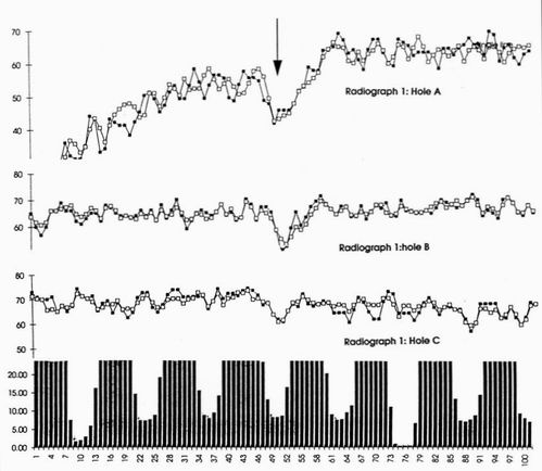
Figure 1. The scanned image of a radiograph along a line crossing a three drilled holes of
A: 0.4, B: 0.3 and C: 0.25 mm diameter drilled holes in 9.6 mm steel. The arrow shows the positions of the hole.
The closed points lie along the scan, the open points are the average of a group of three scans.
The histogram at the bottom shows 1mm lines from a ruler.
Figure 1 shows an actual trace across a 0.4, 0.3 and 0.25 mm diameter holes in a 9.6 mm thick iron slab
obtained from a captured image of a radiograph. The dips in the centre of the figure shows the image
of the hole, the 0.25 mm diameter hole C looks clear enough under the arrow, but is not in fact
significantly different from the larger noise fluctuations such as that near the right of the trace.
Its Probability of Detection is, by any standards, less than 50%. The figure also shows clearly the
fluctuations in the density, whose mean level and spatial frequency may be evaluated. Their
spatial extent is to some extent determined by the film grain size, but more by the correlated
nature of the darkening caused by the highly energised X-ray quanta. The characteristic extent of
the broadening caused by a single X-ray quantum is known as the film unsharpness Uf of the film, and
while the film grain size may be only 0.03 mm, the film unsharpness may increase up to 0.5 mm
for the higher energy X-rays, or gamma rays. The film unsharpness distance is used to define the
edge length of the unit of resolution for the radiographic model. If the mean number of X-ray
quanta falling within this area can be calculated, the statistical spread in intensity over the
area may be modelled analytically as a Gaussian distribution, whose standard distribution
so will be equal to the square root of the
mean number of quanta N,
so =Nl/2.
The actual distribution will be
P(N)=N.(so-2.
exp[ -N2/2so2)].
(1)
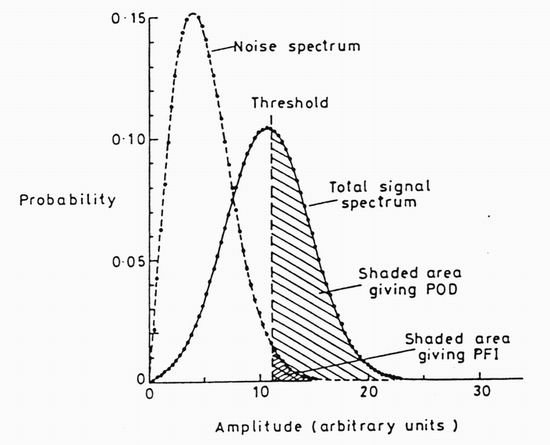
Figure 2. The distribution of pixel intensities after the theory of
reference 2. A fit to the noise distribution is given by the dashed line. The full line
shows the displaced distribution corresponding to the superposition of a signal on to the noise.
The shaded areas above the threshold define the PFI and POD respectively .
This distribution is plotted in figure 2. If a signal caused by a defect causes the mean
number of quanta in the standard area to rise to a signal S corresponding to noise N
and a defect signal So, then the distribution has the Rice probability
P(S) = S.so-2.
exp[ -(S2 - So2)/2s
o2)]Io[SSo(s
o-2)]
(2)
where Io[x] is the zeroth order Bessel function. This distribution is also
plotted in figure 2 for a signal to noise ratio of 2. The standard way to detect a defect would be to
look for an intensity increase well above the mean noise level, as illustrated by the threshold
shown by the arrow in figure 2. If the threshold is denoted by thres then probability that purely
statistical fluctuations in the absence of a defect give this false indication is given by the
integral
PFIo = òT
¥
P(N).dN = 0.5{1-erf[thres/(21/2/so)]}
(3)
shown shaded in figure 2. If a positive signal is present the same threshold gives a higher
probability of detection given by the increased area of the curve beyond the threshold
PODo = òT
¥
P(S).dS = erf[(thres - Dd
/(21/2/so)]
(4)
In radiography the signal may equally correspond to decreased intensity, for example from a dense inclusion.
In this case the integrals must be taken in the opposite direction, and a lower threshold T defined.
If defects of either sense may be present then the two probabilities for positive and negative integral
limits must be added together. A key unknown in these integrals is the threshold T.
It may be estimated from the experimental limit in the differentiation of density changes
which the eye can distinguish, about 5%. However it remains a variable parameter in the present model.
Its choice depends on the application, for example, on how expensive the repair of false indications
compared with the expense of missing a defect. The well-known ROC curves are designed to achieve the
optimal threshold giving the best compromise between missing defects and picking up false indications.
3. Human visual perception
When examining a radiograph the human eye identifies the presence of a defect in a complex way
very different from any simple threshold. Any radiographic interpretation course is designed to train
the future inspector to recognise any given type of defect by example. It is not a quick process,
for actual defects are always different in size, density and shape from one another. Of course
in practice they might appear at any position over a radiograph, or in any one of a series of radiographs.
The brain has to learn to recognise the general features of the object being searched for from a
series of different examples. The eye then scans over the radiograph searching for this
generalised image. The eye has built into its operation an impressive list of options for image analysis.
It is able to work at several levels of resolution simultaneously. Thus even in a situation where
the mean noise level means that many pixels exceed the 5% threshold, if the mean signal changes
over an area encompassing many pixels, the eye is able to integrate over these and pick up the defect
from a single glance at the image. It seems therefore to be able to start work at an extremely
coarse resolution and as we search in more detail continuously reduce the search area covered by our eye.
Almost all real radiographs have smooth intensity changes across their area caused by the
differing X-ray path lengths. The eye hardly sees these, and is able to pick out contrast details
much smaller than the actual density changes across the extent of the radiograph. The eye is
particularly good at searching for a feature which it has previously seen and remembered. We all
recognise how well we can search some text for a particular word. This "template matching" mode
can be performed by the eye simultaneously for several different templates.
Neural network receptive field methods are able to work in exactly this mode. They sweep a
small field of view over the radiograph, mimicking the human fovea, and present the pixels
within the receptive field to a neural network trained to give a large output when a defect
of a given type is presented to it. However the eye does not scan in any such systematic way.
A defect, obvious to the eye when pointed out afterwards, may often be missed during the original
radiographic interpretation. It is not just the human factors of fatigue, boredom or
carelessness which cause the error, although these are all important, for even a fresh
well-motivated inspector will not perform as an ideal model predicts. It is rather the intrinsic
difficulty that humans have in behaving like computers - performing the lengthy, repetitive task
of scanning every section of the radiograph and searching for one of any number of possible types,
sizes and shapes of defect. A key factor is experience - it is a well known fact that
radiographic inspectors see one gauge finer wire in an Image Quality Indicator than do raw recruits.
This paper takes a pragmatic approach of attempting to validate its POD calculations by
simulating radiographs together with noise, defects and IQI's, and asking operators to compare
their own performance with that of the model. The human factors are thus included at the same
time as the model based factors. The model doubles as a training tool in its own right by giving
operators a view of the size, contrast and sharpness of typical defects that they need to be able to identify.
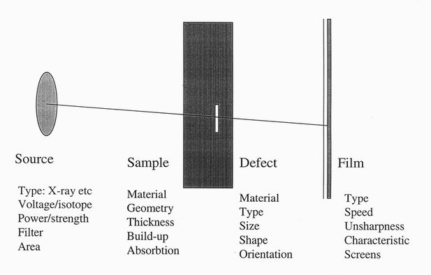
Figure 3.The principle factors which need to be taken into account in evaluating a
defect Probability of Detection using X-radiography.
4. The physics of the radiographic model
Figure 3 shows the key factors which need to be included in any radiographic simulation.
It is not practical to build in all the detail which should ideally be included.
Appendix 1 shows the parameters which have been included in the present code XPOSE.
The parameters are entered in from a series of menus and toggled in (T), entered as variables
(V), or measured or interpolated from experimental data (E). A key objective of the
code is that the derivation of all data used are clear and referenced to their source, and that
the data finally used are, at least optionally, displayed to the user.
Source
There are important differences between X-ray and gamma sources in radiography. An X-ray set
usually has a variable electron acceleration voltage which becomes a key factor in determining
exposure and contrast. The energy spectrum of the X-rays produced depends on this energy and also
on the target material. There is generally a set of monochromatic lines produced by electrons
dropping back into an empty deep atomic orbital whose occupant had been ejected by the X-ray.
These transitions are superimposed on a continuous distribution, the Bremsstrahlung or
slowing down radiation, produced as the electrons are stopped in the target. Tungsten is by far
the most commonly used isotope in industrial radiography, and its use is assumed in this study.
The intensity of X-rays emitted by a tungsten target being hit by electrons of a given current
and voltage is assumed to be the same. The distribution with voltage is presently taken from
the PANTEC source data, and is assumed to be independent of current so that exposures are measured
in ampere-hours. Filters are widely used in X-ray sources to remove low energy X-rays which,
because of high multiple scattering, reduce the effective contrast. The emitted X-ray flux
will be assumed to be measured with the filter in place.
Isotope sources are used for thicker specimens when electromagnetic quanta of higher energy,
gamma rays are needed to give adequate penetration. These sources emit one or more gamma rays
which together are assumed to have some characteristic mean energy. This energy remains fixed
with time, although its intensity will decay with an exponential fall-off with a time constant
depending on the half-life of the source. Since there is no way of varying the gamma ray energy,
there is no analogue of the X-ray voltage, nor of the X-ray current. The intensity of gamma ray
sources is defined simply from the number of disintegrations per second.
Betatron sources are relatively portable accelerators than can produce very hard gamma rays
of several MeV energies capable of penetrating many inches of steel or metres of concrete.
Again the voltage is effectively fixed.
Sample
The sample material effects an X-radiograph in several respects. The absorption of X-rays is
material dependent, and this in turn effects the recommended voltage, the exposure curve, and the
number of X-rays reaching the film. Table 6.9 from Halmshaw's book gives recommended X-ray voltages
as a function of thickness for iron and aluminium. Figure 4 shows the graph of this function as used.
A warning is given if the sample thicknesses lies outside the recommended range of suitability,
either for X-rays or for any chosen gamma source.
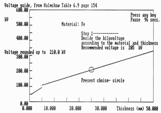
Figure 4. The linear relationship used by Halmshaw[1] to evaluate an appropriate X-ray
voltage for a given sample thickness of iron. The circle shows the operating position.
An iron plate scatters X-rays strongly enough that the change of an X-ray being scattered rather
than absorbed is by no means negligible. This means that the geometric image of any defect can
be degraded by X-rays which enter its shadow. This "build up factor" is defined as the ratio of
the total X-ray intensity at the film divided by the intensity arising from X-rays which arrive
at the film directly. The factor is therefore greater than unity, and can rise to large values
so that the majority of the observed X-ray intensity comes not from the image forming direct
radiation, but from the diffuse scattered intensity. The effect increases with material thickness,
and with its atomic number which effects its scattering cross section. Since low energy radiation
is more readily scattered build up increases with decreasing X-ray energy. Figure 5 shows the
measured data used in the program from Halmshaw. The lines through the data are quadratic fits
to the data at each thickness, whose coefficients have been fitted as a function of energy so that
the build up may be interpolated at any voltage or energy. Similar data exists for aluminium plates,
and for iron plates under gamma radiation. These data are only relevant for the simple slab geometry.
However a cylindrical geometry may be approximated by that of two flat plates each equal to the wall
thickness and separated by the diameter of the cylinder. The scattering from the upper plate may be
considered an isotropic scatterer on to the lower plate. There exists good data on these effects
for iron and aluminium. For this reason, a given thickness of most other materials is expressed
in terms of an equivalent thickness of one of these two standard materials. The conversion factors
are derived from the table originating from Kodak quoted in the Welding Institute Handbook [6].

Figure 5. The measured build up factor (BUF) as a function of thickness for various X-ray
voltages from Halmshaw [1]. The lines shows the double variable interpolation to his data.
The circle shows the current operating position.
The absorption cross section has several components and needs to be considered as a function of
both X-ray energy, or gamma ray source, and thickness. These have been tabulated by Halmshaw and
figure 6 shows the interpolated fit to these data for iron.
Figure 6. The measured material absorption as a function of thickness for various X-ray
voltages from Halmshaw [1]. Again the lines shows the double variable interpolation to his data
and the circle shows the current operating position.
Figure 7. The sample geometries detailed in the model.
The sample geometry is important in that it affects the thickness of the material through which the
X-ray or gamma ray beam must pass compared to the thickness relevant to the calculation of the
resolution or geometric unsharpness. The geometries considered are displayed in figure 7.
For the simple slab geometry both thicknesses are equal to the basic wall thickness t,
as they are for "Single Wall Single Image", "Film Inside Source Outside" or "Film Outside Source Inside"
geometries. However the "Double Wall Single Image" geometry has an effective absorption thickness
tabs = 2t , twice the wall thickness, while the resolution thickness remains equal
to the wall thickness tres = t. In the "Double Wall Double Image" geometry the
absorption thickness is again twice the wall thickness, but the resolution thickness is equal to
the pipe outer diameter tres.
Figure 8. The definition of a single angled cuboid defect, with respect to conventional axes
in a weld.
Defects
The modelling of defects near the limit of visibility need not be taken to the same degree of detail
as would be possible for more clearly seen defects. For this reason only assemblies of cuboidal defects
are presently considered. With these shapes the necessary convolution of the Gaussian unsharpness
over the defect volume may be performed analytically. Different types of defect are then defined in
terms of length and depth aspect ratios, orientation and number of components. A single defect component
is defined as in figure 8 by its length along the weld x, its depth or "gape" y, its
width across the weld z, and the angle q defining the
orientation of the defect x axis in the plane along and perpendicular to the weld. In order to
compare and visualise defects of different type the effective diameter of the sphere of equivalent volume
is taken as the size standard. The two further definable parameters are the aspect ratio along the weld
ax=x/y and its aspect ratio across the weld ax=z/y. The volume and effective
diameter of a cluster of n such defects is therefore
V = nxyz = naxazy3 = (1/6)np
deff3.
(5)
Figure 9. Defect sizes are defined in terms of the diameter of the sphere deff having the same
volume as the composite defect.
The X-ray transmission through a single oriented cuboidal void is only dependent on the path length
along the beam, and not on the material distribution along the beam. It is therefore to make an
approximation that cuboids of area 2a.2b orientated at the angle q
to the X-ray beam may be transformed into cuboids of area 2aeffx2beff
as illustrated in figure 10. A sensible definition for the transformed volume is
aeff = nxyz = 1/(cos q/a +
sin q/b ) beff = b cos
q +a sin q
(6)
This definition keeps the area precisely correct and has the correct limits for the extreme
angles of q9 =0 and 90o when the X-ray beam
is perpendicular or along to the defect length. The approximation is good for high aspect ratio
b/a, as for example the case b/a=20 in the figure. For moderate aspect ratios it works
less well as it fails to describe the true trapesoidal form of the transmission. However the
differences are likely to be unimportant in the practical case of defects at the limit of visibility
when geometric unsharpness broadens the tapesoidal edges of the profile.
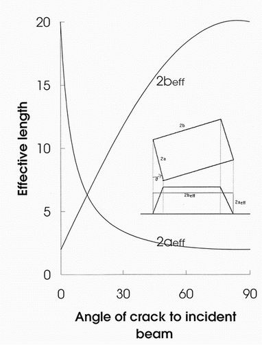
Figure 10. Cuboid defects whose normal lies at an angle q9 =0
to the X-ray beam axis are transformed into cuboids in the plane perpendicular to the beam with
effective length 2beff and gape 2aeff. The true trapesoidal path
length variation is turned into a rectangular one. The figure shows the variation of these as a
function of angle for b/a=20.
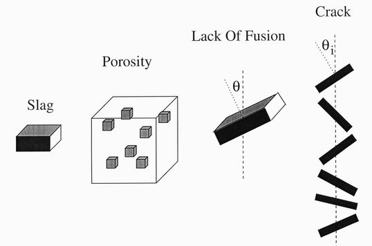
Figure 11. The types of flaw considered in this study.
The present study is limited to just four generic types of flaw, whose parameters are collected
together in table 1.
i) Slag inclusions are a common type of flaw, and being volumetric are much less likely to
initiate failure than the various types of crack. They are typically rectangular in section
elongated along the axis of the weld. Our model will assume a single cuboid n= 1 with a square
section of variable gape and width y, az=l, elongated along the weld by a length aspect
ratio ax=4. These parameters may of course be changed within the definition file.
ii) Porosity is common in the centre of welds and being volumetric is again relatively benign
in its ability to initiate failure. The key parameter is the mean width y of the cuboid
individual pores making up the volume of porosity. The area of porosity is assumed to be 5 times
the pore width along, across and down the weld bx=5,by=5,bz=5
and to have a 12.5% volume fraction so that n=12.
iii) Lack of Fusion cracks occur along the boundaries between the weld material and the
workpiece when fusion has been incomplete. They are serious flaws as their edges contain stress
concentrations which may initiate crack growth leading to failure. They are usually flat in
cross section in the plane of the weld face. Our model assumes a gape width y with factor 10
aspect ratio both along and transverse to the weld ax=10,az=10.
They are usually orientated at a known angle to the X-ray beam, so their visibility depends
crucially on the angle of the normal to the crack to that of the X-ray beam. An angle of 70�
is typical for conventional "double V" welds.
iv) Rough cracks occur when excessive thermal stresses cause metal within the weld or the
heat affected zone to fracture. They are at once most serious, and difficult to model, since their
shape and orientation are highly variable. However they share a general feature of having many facets
at different angles, and the present model assumes 10 facets with a specified mean angle, and
spread of angles around this mean. It assumes a variable gape width y, an aspect ratio
along the weld ax=10, an aspect ratio across the weld azz=10,
a mean facet angle q of 70�, and 10 individual facets
with a angular spread dq, of 20�. Figure 11 shows a
Lack of Fusion crack some 50x1O mm. in area with a gape of 1 mm, compared with its model.
Table 1. The definitions of the assumed defect types
| Type | ax | az | q |
dq | n | bx | by | bz | deff |
| Slag | 4 | 1 | 0 | 0 | 1 | 1 | 1 | 1 |
(24/p)1/3y |
| Pores | 1 | 1 | 0 | 0 | 12 | 5 | 5 | 5 |
(125/p)1/3y |
| LOF | 10 | 10 | 70o | 0 | 1 | 1 | 1 | 1 |
(600/p)1/3y |
| Crack | 10 | 10 | 70o | 20o | 10 | 1 | 1 | 1 |
(600/p)1/3y |
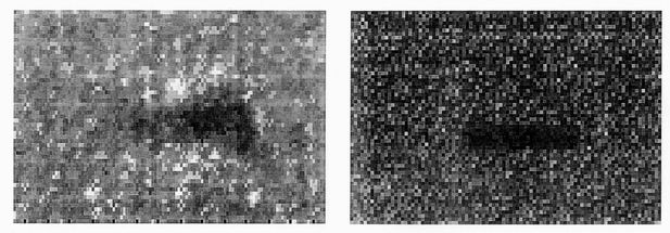
Figure 12. On the left is an X-radiograph of a slag inclusion and on the right its simulation.
The simulation fails to show the film grain speckle or the detailed shape of the inclusion.
Film
X-ray photographic film responds to a given flux of X-ray quanta in a complicated way defined by
film density, or logarithm to the base 10 of the light transmission after development, as a function
of the logarithm of the exposure. This "characteristic curve" is strictly unique to a particular make
and speed of film. However the main parameter is the speed, which mainly affects the position of the
curve along the exposure axis, and only to a lesser extent effects the shape of the curve.
The speeds are obtained from Halmshaw Table 5.1 page 98 [1]. Figure 13 shows the very precise fits
achieved to the Kodak MX and CX films which are most commonly used. The function used is a
quadratic polynomial divided into two regions, together with a constant "fog" term. These are
fitted to actual data from the manufacturers data sheets as the program is run.
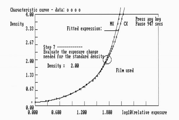
Figure 13. The exposure curves for Kodak MX and CX X-ray films. The points are from the
manufacturers product sheets, while the lines show the fitted function. The circle shows the
chosen working position. The contrast factor, needed in the POD calculation is evaluated by
numerical differentiation of the fitted curve at the working position
5. Unsharpness: the contributions to the spatial resolution
The evaluation of the unsharpness, or spatial resolution, in the radiograph is a prerequisite
to both the simulation of the radiograph and the defect probability of detection. The total
unsharpness is derived by convoluting the unsharpness terms originating from the film, from
the X-ray source size, and from the geometry as defined by the source to sample and sample to
film distances. The present model assumes that all these contributions may be approximated by
Gaussian distributions.
uI = (2psi2)-0.5
exp(-2x2/si2
(7)
where x is any linear dimension. This enables them to be described by a single number,
the full width at half height of the Gaussian distribution, FWHHj =(21oge2)
1/2si ,
and to convolute the various contributions by summing squares and taking the square root.
As we shall see later it also allows the convolution with a rectangular defect to be performed analytically.
Film
The film unsharpness Uf is a function of the voltage of the X or gamma rays,
and figure 14 shows the film unsharpness measured by Halmshaw[l].
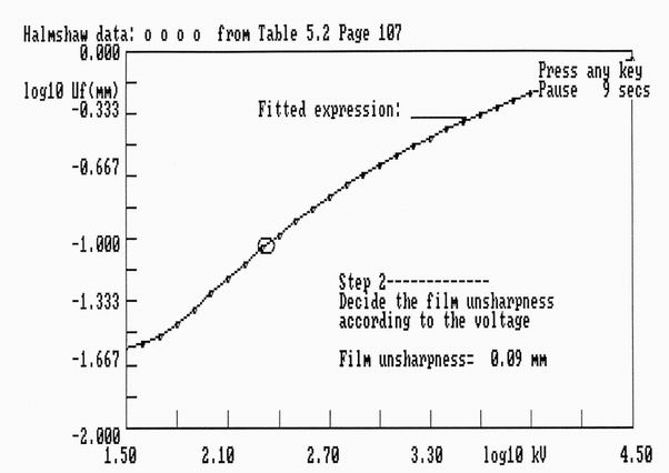
Figure 14. The film unsharpness Uf as measured by Halmshaw[1] and fitted in the model.
The circle shows the currentlfcuboidefy assumed value.
Source
A second important contribution is the source size unsharpness Us. This is usually
evaluated according to the most pessimistic case from the diagonal length of the X-ray target or
gamma source dimensions
us = [ Usource_length2 +
Usource_width2 ]1/2
(8)
A better approximation can be derived experimentally by measuring the source function by using a
pinhole geometry and evaluating the best fitting us.
Geometric
It is conventional to assume that the defect or IQI lies close to the upper surface of the sample,
where the geometric unsharpness is largest. The overall geometric unsharpness is then calculated
for a given source to film distance sfd with the defect to film distance equal to the sample thickness t
ug = [ Us/)sfd/t-1)
(9)
Alternatively if the geometric unsharpness is to be specified then a minimum source to film distance
sfd may be calculated from
sfd = t.[1+ Us/Ug]
(10)
The program gives a visual demonstration of the three unsharpness distances Us,
Ug , and Uf, as illustrated in figure 15. The total unsharpness may be
simply evaluated by quadrature within the Gaussian approximation.
In order to speed up the simulation the full random noise pattern is calculated only over a
limited area of the screen, say just a 32x32 area from the 640x340 pixels available. This area
may then be copied over the rest of the area of the simulation with little loss in the perception
of randomness.
The 32x32 pixel area is also used to demonstrate the geometric unsharpness. An absorption in the
form of a Gaussian distribution with a full width at half height equal to the calculated geometric
unsharpness is superimposed on the small area of noise. The image is thus that of a fully absorbing
pinhead. This gives a visual impression of the resolution broadening expected around any feature
in the radiograph.
The image of a defect as seen on the simulated radiograph takes the form of an array of exponential
absorption factors appropriate to the path length though the specimen at each point, convoluted
with this Gaussian resolution function. The defects in the present version are assumed to be void
cuboids with axes along the plane of the sample. It is then possible to perform the resolution
convolution analytically. Suppose the cuboid has depth dx
and lies in a medium with an absorption constant m and a thickness t. The intensity I
will be attenuated in the material as a function of depth x according to
I = Ioexp(-mx)
(12)
change in intensity DI/ caused by the defect of
path length DI/ will be
DI/I = -mDx
(13)
The relative change in intensity DI/ is converted in
the film to a density change DD/ depending on the gradient
of the characteristic curve for the particular film and exposure Gd according to
DI/I = -DD/
(log10Gd
(14)
Having evaluated this change in absorption it is necessary to perform a convolution with the
Gaussian unsharpness function discussed above. For cuboid defects this integral becomes analytic being,
at each point, the integral of a Gaussian between the two limits formed by the edges of the defect
which takes the form of the error function. The final intensity at pixel i,j is given for a
defect of width w and length l by
C= 0.5{erf[w-i.Uf/s] -i.Uf/s -erf[-w - i.Uf/s]}
.0.5{erf[1-j.Uf/s] -erf[-1 -j.Uf/s]}
(15)
The differential change in film density caused by the defect will then be according to Halmshaw's
equation 2.17, and including the build up factor B
Dd = -0.4344.C.m.Gdm
dx/B
(16)
This represents the basic equation for the density change expected from a given defect.
The optional simulation of an Image Quality Indicator (IQI) is an important aspect of the
radiographic simulation as it is an important option in any real radiograph. The two most suitable IQIs
are chosen from the list of the most commonly available types as shown in table 2. Only conventional
multi-wire gauges composed of 6 or 8 wires about 80 mm long encased in a plastic
case are considered at present. These indicators are composed of wires of iron, aluminium or copper,
and the optimum wire diameter is either specified or evaluated from the specified thickness sensitivity.
The actual wire thickness must be adjusted according to the material if it is not one of the
standard materials, iron, aluminium or copper. The next lowest diameter wire gauge available
is selected from this list, and the two most suitable IQIs chosen from the list of those available
by choosing that which has the desired wire gauge most nearly in the middle of the IQI. The image of
each wire is evaluated by choosing a width across the image of the wire that will be sufficient
to include the geometric unsharpness, with pixels equal to the film unsharpness. The convolution
of the Gaussian geometric unsharpness with the arc length distribution across the cylindrical
wire is then evaluated and stored in an array. This convolution is unchanged down the length of
the wire so that it is possible to evaluate new random pixels at each pixel along the length of
the wire from the same stored array of mean intensities. A typical simulation is shown in figure 16.
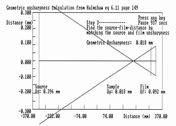
Figure 15. A radiographic simulation of a typical series of slag-like cuboid defects
with increasing size in a 25 mm steel plate. The marker lines are centred on the defect and
indicate its size. The smaller defects are not visible in the simulation but the larger ones
can just be seen. The inset in the top left corner illustrates the total unsharpness.
The numbers indicate the 7 wires of the IQI DIN54.109, only some of which can be seen.
7. The evaluation of the Probability of Detection and Probability of False Indication
The single pixel probability of detection equations were given earlier. Once again the necessary
function is the integral of a Gaussian between fixed limits and may be expressed analytically as an
error function. The area of the Gaussian centred on the mean brightness from the threshold to
infinity gives the single pixel PODo and probability of false indication PFIo
per pixel with area equal to the film unsharpness which were given in equations 3 and 4. The
threshold value thres needs to be specified. It represents the density change which can be
perceived as distinct to the eye, when presented in a series of isolated pixels with a noise distribution
characterised by the deviation s. Halmshaw (p237) [1]
mentions that a 5% luminance difference, corresponding to a 0.02 film density difference is the
sort of performance within the capabilities of the human eye under good film viewing conditions.
We follow him in adopting 0.02 as the default threshold. However it must be admitted that this
crucial factor is somewhat subjective.
It is well known that the eye is sensitive to much smaller density variations if there are many
adjacent pixels with the same mean density difference. The eye is able to integrate over those areas
of the image having the same mean density - say inside and outside the image of an extended defect.
The effect is the same as if the pixel size had been increased by appropriate averaging to give a
higher mean number of quanta per pixels and consequently a lower standard deviation
s. However averaging pixels numerically over some
area is no solution since the resolution will be degraded and a group of pixels may or may not appear
above the threshold depending on whether the averaging length spans the defect edge or not.
This problem does not arise with the method used, which is based on that used in the corresponding
ultrasonic code by Ogilvy[2]. An odd number n.m of adjacent pixels is considered, and the POD
and PFI is evaluated for every possible choice of central pixel. The defect is accepted if all n.m
adjacent single pixel probabilities Pi,j individually exceed the threshold.
Similarly a false indication is declared if all the n.m adjacent probabilities exceed the
pure noise distribution threshold. Thus
PFImxmy= 1 - { 1 - [1 - (1-f)M-m] }n }N-n
(17)
PODmxmy= 1 - { 1 - Pk=0 to n-1
[1 - Pi=1 to M-m
(1 - Pl=1 to m-1 ) ] }
(18)
Choosing the best values to choose for the averaging distances n,m is a matter for some discussion.
The eye tends to choose that distance corresponding to the smallest object for which it is searching,
whatever the size of the defect actually seen. The conclusion is that the distances n,m should be
fixed to correspond with the smallest defect detectable. However it would be reasonable to enlarge
the averaging dimensions as the size of the defect being searched for increases. Thus a human might
be imagined to search over an image several times, each time looking for a different size of defect
and performing a mental averaging corresponding to this size. The problem with the second approach
is that it leads to a much more rapid increase in the probability of detection with defect size than
is actually observed. The method presently uses a fixed averaging size of three times the film unsharpness.
The POD curve for the cuboid defects in 25 mm steel illustrated in figure 17 is shown by the points
in figure 18. It is seen be close to zero for effective diameters below 0.4 mm then to rise quite
sharply at around 0.6 mm rising to essentially 100% by 1 mm.
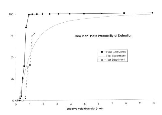
Figure 17. The points show the calculated probability of detection as a function of defect size
for cuboid defects in 25 mm thick steel. The full line shows the experimental results for
radiography by Forli [9]. The crosses and dashed line show experimental POD measurements from
human trials using radiographic simulations.
8. A comparison with experimental POD results
There exists a considerable literature of experimental test data on Probability of Detection of
defects using X-radiography. This has been gathered into a computerised database by M Wall [8]. As an
example of the type of comparison which may be made, the feint line in figure 17 shows a portion
of the results of Forli [9]. Although this work covers a range of samples, the results are not inappropriate
for radiography of 25 mm plates. There is quite a serious discrepancy between this curve and the
calculated results for 25 mm plate shown by the points. In fact the defect size where the defect
may first be observed in favourable cases is seen in both cases to be around 4 mm. However while
the calculated POD rises rapidly to close to 100%, the experimental curve saturates much more slowly.
It is believed that the differences between the two curves are largely accounted for by the human factors.
9. The quantitative analysis of a scanned experimental radiograph
An experimental test of the method has been provided by a radiograph of a test specimen containing
four drilled holes covering the limit of expected visibility which had been developed to establish a
test procedure for an important inspection application. The procedure was as follows:
| X-ray set: | Philips PANTEC |
| Source size: | 0.4 mm |
| Exposure: | 8.8 mA.min |
| SFD: | 600 mm |
| Film: | Kodac MX |
The specimen was of steel 9.6 mm thick with cylindrical holes drilled:
| Label | Size | Human | XPOD |
| A: | 0.4 mm diameter: 0.4 mm depth | 90% | 95% |
| B: | 0.3 mm diameter: 0.3 mm depth | 60% | 45% |
| C: | 0.25 mm diameter: 0.25 mm depth | 25% | 19% |
A radiograph covering these holes was taken. The percentages on the right were a human assessment of
the probability of detection of these holes from a careful viewing of the original radiograph under
ideal conditions. The radiograph was then scanned through a video camera and captured on an image
analysis system. It is not possible to display here the original radiograph with anything like
the required quality, but figure 1 showed the direct scans of the image intensity. The heavily
sloping background illustrates the problems of naive methods such as taking a simple threshold at the
lower limit of the noise and looking for dips below this. The POD values obtained by the program
are shown above. They are seen follow the human estimates reasonably well. We would not claim any
higher degree of accuracy in POD than the 10 to 20 % precision obtained here.
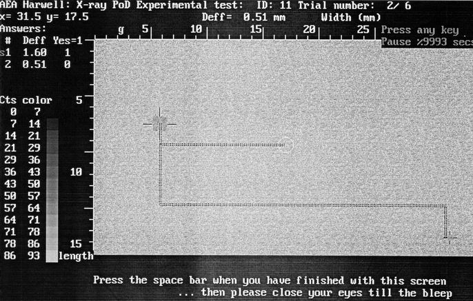
Figure 18. The screen display from the experimental trial including human factors. The dark
square to the upper left shows a clear defect detected by moving the cursor as shown by the parallel
dashed lines. The defect in the lower right hand corner was just missed by the cursors .
10. An experimental way of including human factors
The radiographic simulation can easily be adapted to provide an experimental tool for the measurement
of the human POD (and PFI) for particular defects under any specified circumstances. An average number
of defects per display is specified and a random number of defects within a defined effective diameter
range is simulated and presented onto the screen for examination by the inspector. Inspectors can
move a cursor around the screen as shown in figure 18. They may press ENTER at any time they choose
and if the cursor lies within a specified distance of the defect a HIT will be scored. If no defect
exists there, a MISS indication will be scored. The inspectors are not told how many defects they are
searching for, and they must themselves decide when to press END to indicated the completed inspection
of the screen. After a specified number, say 10 screens, the HIT and MISS totals are recorded and
plotted as a function of the actual defect effective diameter. The crosses in figure 17 shows such
an experimental POD plot obtained from several inspectors. Some were trained X-radiographers, but
most were physicists working in an NDT department. There was no significant difference between the
two sets of people. Most people obtained a similar performance, but they were all significally below
the calculated POD curve, and fall closer to the experimental curve.
11. Conclusions
The XPOD model described here provides a path from a given radiographic procedure, to the simulated
radiograph of an assumed defect, and to its POD and PFI. Validation through IQIs give confidence that
the method gives a good indication of POD, although there are uncertain factors in the calculation
such as the assumed film density threshold, and the averaging distance in the Ogilvy correlation.
Ultimately these need to be settle by more extensive validation. Without doubt, these calculated POD
curves do not correspond well with experimental trials. We believe much of the difference can be
accounted for by human factors. This is especially true for larger defects whose existance is obvious
when pointed out but which are nevertheless sometimes missed in practice. A experimental method of
measuring human POD from simulated radiographs has been developed.
References
[1]R Halmshaw, "Industrial Radiology, Theory and Practice", Applied Science Publishers Ltd 1982
[2]J A Ogilvy AEA APS 0365, Feb 1993, NDT International, 1994
[3]O Forli,"Reliability of radiography and ultrasonic testing", Procs.5th NDT Symposium, Esbo, Finland, 1990
[4]T A Gray and R B Thompson, "Use of models to predict ultrasonic NDT reliability", Rev.Proc.QNDE, 7B, 1737-1744, Plenum New York, 1988.
[5]Metals Handbook, 9th Edition, Vol 17, "nondestructive Evaluation and Quality Control",
"Models of Predicting NDE Reliability", p 702 - 716
[6]The Welding Institute Course Handbook "Practical Radiography NDT20 1996
[7]Murgatroyd R L et al: Human Reliability in Inspection: Results of Action 7 of PISC III programme, 1994
[8]M Wall, APS POD Database, April 1992, Unpublished
[9]O Forli, NDT SYMPOSffiT ESBO, Finland 1990-08-26...28, Nordest, Finlands, Svetstekniska
Forening NDT-KOMMITEEN.