Abstract
The smooth non-linear mapping between one multivariate function and another which both preserves the local details at corresponding points in the map and also minimises the complexity of the map is the basis of elastic matching. Its roots in two—dimensional image mapping will be described, but many of its methods are best appreciated in one dimension, which has several important applications in its own right. The general procedures and methods for enhancing success will be described together with applications to gas chromatography, static and dynamic signature recognition, and face recognition.

1. Introduction
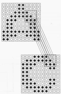
The biological basis of elastic matching was described by Beinenstock in terms of the structure of the human visual cortex. Figure 1 after his paper describes the type of connections which are thought to exist between different layers in our visual cortex. When corresponding neurons on a template layer (above) and test layer (below), indicated by the heavy line, have both a common firing mode (black or white) and also a common set of nearest neighbour enviromnent of firing pattems then a reinforcement mechanism is assumed to apply and the connections between the two layers are reinforced. Figure 2 shows the type of nearest neighbour neuronal circuit which Von der Marlsburg and Bienenstock [2] describe. Two adjacent firing neurons (black) send their signals both to their near neighbours, and to a second similar layer of neurons. A four-neuron loop is therefore formed when both emitter and receptor neurons have the same firing mode and so would tend through Hopfield’s Hebbian learning reinforce the connections between them. The common nearest neighbour environment may readily be generalised to include the more distant surroundings of the central connection, and less precise matchings. In general a good match can be specified by high correlations between the connected regions of the template and test functions.

Figure 1. The type of links suggested to occur in aeyacent layers ofthe human brain by Beinenstock[1]. Particular neurons in the two layer (as joined by the full line) have several neighbours with similar pixels on each layer, giving a series of reinforcing circuits.

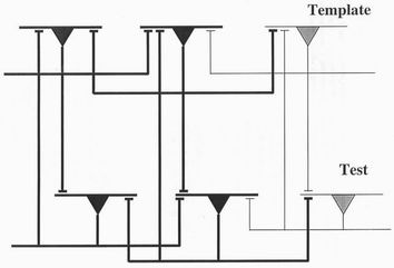
Figure 2. The neuronal picture of adjacent pixels (black or white) in the two layers storing the prototype and test images. Links from the axon of each cell connect both with adjacent layers and with near neighbours in the same layer. A four-neuron circuit of neurons with a similar firing pattern can therefore be established.

For example corresponding positions in a hand-written signatures could include correlations between the spatial positions, and also the pen timings, pen velocities, and tip pressures. This type of correlation mapping is invariant to spatial displacements between the objects and at least partly invariant to rotations and scale changes. The second fundamental principle of a good mapping is that it should be appropriately simple. In many practical cases nearly perfect local correlations can be achieved between points in the two functions which are nevertheless incorrectly matched. For example in signature recognition of the name "Bill Full", the both words end with the same "...ll" sequence. As illustrated in figure 3, it is likely that there will be good local correlations from any one example in the template to both examples in the test signature. The ambiguity can be minimised by including more distant correlations, but it can more easily be removed by requiring that the matching transformation between the two signatures be a smooth one. The match to the correct position gives a smooth function, while the match to the second requires a sudden gap.

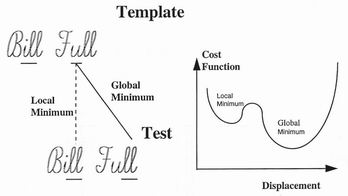
Figure 3. Two hand-written signatures being compared. Any correlations existing between the marked "ll" sequence arebound to be echoed in the false connection which therefore represents a local correlation minimum.

The name elastic matching derives from the technique of finding a good linear match between two images by printing the test image on a transparent elastic sheet, and stretching the sheet until the template and test images optimally overlap. The technique is readily generalised to functions of higher or lower dimensionality and to non-linear mappings of all kinds. The concept leads naturally to a particular criterion for a possible mapping - that which leads to the minimum elastic strain energy within the elastic sheet. According to Hooke's law for a perfectly elastic medium, the force F when an elastic object of length x is stretched by a length dx is F=Ydx, and the elastic strain energy is E=Ydx2/2. Consider a template function array x_A(i) compared to a test function x_B(j), connected by a link array L(i) which connects the ith point on the A array with the j=L(i)th point in the B array. The total elastic energy is then seen to be proportional to E=Y S_i (x_A(i)² - x_B(L(i))² )/2. Thus the minimum elastic energy corresponds to the minimum least squares differences between the points on the template function and the corresponding matched ` points on the test function. Unfortunately such a simple algorithm is not invariant to even translational displacement which will certainly stretch the elastic sheet! Appropriate preprocessing to define objects with respect to their centres of gravity, their principal axes, and their principal radii could restore to the elastic sheet its objective of looking for a smooth set of matching connections, but such an approach will never be optimal as it will always try to remove any type of distortion between the functions. What is needed is a function which is neutral to smooth elastic distortions but which penalises the spatially sharp distortions produced by incorrect linkages.

2. Obtaining a good match - a one dimensional example
It is usually easy to define, as in the above section, the criteria by which a satisfactory elastic match can be judged. It is even easier for the human eye to judge a successful match, and note any inconsistencies. The problem is how to achieve it. An important one-dimensional example of the need for elastic matching occurs in gas chromatography. A small sample of say peppermint to be assessed against a standard sample is vaporised and the gas passed through a long chromatograph whose output is a series of peaks describing the arrival time of different molecular species. For the purpose of this discussion it is assumed that the raw data is separated into a series of discrete peaks as similar height as a function of the retention time through the chromatograph. Figure 4 shows such a spectrum for a template sample A (upper) and a test sample B (lower). The problems of connecting corresponding peaks in the two spectra are evident. There is a considerable displacement between the main groupings of peaks which the eye is quick to see in both patterns. However the displacement is not constant or even linearly changing along the spectra. Some template spectrum peaks have no corresponding partner in the test spectrum - we call these "dangling" peaks. Some test spectrum peaks do not appear in the template - "rogue" peaks. Some peaks in the template would like to connect to a single peak in the test spectrum - "Multiple" peaks.

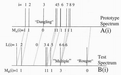
Figure 4. Two gas chromatography spectra being compared. Peaks i in the prototype are linked in to peaks L(i) in the test. Various types of mismatch are shown. The arrays N_A(i) and N_B(j) will be used to define a cost energy.

It is instructive to consider how the eye functions when presented with such a pair of spectra. First it searches for the most distinctive cluster of peaks — distinctive because its central peak has correlations with those in its near neighbourhood that are not common in the spectrum. The eye then searches in the test spectrum for a similar cluster. If it finds one, then the eye mentally draws the first link between the corresponding central peaks. The process can then be repeated for the second most distinctive cluster of peaks. If the two links are correct then an approximate mapping is established and if the mapping is at all linear it will often be easy to add other links. If the mapping is more non-linear then the process of searching for distinctive clusters of peaks will have to be continued within the regions of the spectrum between the first links identified. The problems arise when some of the early links were incorrectly made. Lack of any exact match, even with the correct links, can easily lead to an initially incorrect assignment. This is where the eye brings in the elastic sheet. It is able S to size up both spectra as a whole and favour those altemative links where the local stretching of the sheet is minimised. In a complex pair of spectra with many apparently similar local clusters, none . perfectly matching, the skilled eye begins the process which our methods attempts to simulate - that of trying out a wide range of possible connections, weighing up the balance of local correlations and distortions, and slowly settling down on those connections which show most promise.

3. The quantitative description of local correlation
The correlation and distortion concepts may be related by considering each as an elastic energy. The correlation energy representing the elastic energy required to map the environment of the central peak of one local cluster of peaks in the template, when linked to that of another in the test spectrum. The distortion energy is the contribution to the elastic energy of the total mapping from the chosen linkage. . Consider two sets of gas chromatography peak positions, a template spectrum composed of N_A peaks of intensity y A(i) at times t_A(i), and a test spectrum with N_B peaks y_B(j) at times t_B(j). Suppose a current set of linkages between the two spectra j=L(i). The correlation energy may then be written as illustrated in figure 5 as

E_corr = S_i=1,NA S_{k=-ncorr,ncorr} [ X_A(i) - X_A(i+k) - X_B(L(i)) + X_B(L(i+k))]²

where the sum over i runs over all the peaks and the sum over k runs over the n_corr peaks on either side of the peaks i in spectrum A or L(i), the linked peak to i in spectrum B. The correlation energy as so defined is proportional to the elastic deformation energy needed to transform a map of the immediate neighbourhood of a chosen peak in the prototype into that of its linked partner in the test spectrum. Similar correlation terms can be defined for peak intensity in gas chromatography, for variables such as the y position, the timing or pressure of a pen stroke, or for the non—positional variables of a circular arc.

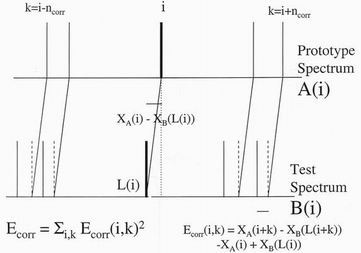
Figure 5. The correlation energy between two linked peaks. It is the sum over neighbouring peaks i+k of the their displacements relative to the displacement of the chosen peak i.

4. The quantitative description of local distortion
The distortion energy term needs to be related, not to the elastic energy of distorting one spectrum into another, but to the extra elastic energy needed to make the distortion over the best current measure of a smooth distortion between them. For this purpose a distortion vector x_D(i) is defined which may be evaluated for a given set of links from the average difference between linked points over the immediate neighbourhood on either side of the ith peak. The distortion energy term is linked to the extra elastic energy needed to distort the points in the prototype spectrum into linked points in the test spectrum. The first step in evaluating this energy is to calculated a "distortion vector" averaged over the n_dist lines on either side of the chosen line i

x_D(i) = S_{k=-ndist,ndist} x_A(i+k) - x_B(L(i+k)).

This array, together with a similar y array in two dimensional problems, can then be used in the evaluation of a distortion energy

E_dist = S_i=1,NA [ x_A(i) - x_B(L(i)) - x_D(i)]².

Such an energy term will then penalise the difference between the actual linked ordinates on the two spectra and their average values.

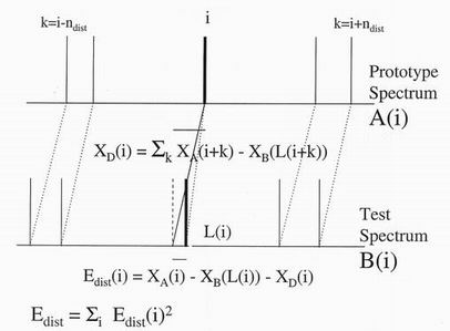
Figure 6. The distortion vector at peak i is the mean displacement over neighbouring peaks i+k. The distortion energy between two linked peaks is the sum of the squared differences between the actual displacements and the distortion vectors.

5. Matching all the links
One of the tasks the eye is good at, is spotting, and making due allowance for, the inevitable links that will never match. These include the "dangle" links when peaks present in the prototype not matched by any in the test, unlinked "rogue" peaks present only in the test and "multiple" links when two or more peaks in the prototype connect to a single peak in the test. The matching process must encourage a one—to-one mapping where best and allow for dangle, rogue and multiple links when these are necessary. These objectives are satisfied by defining two multiplicity arrays m_A(i) and m_M(j) defining the number of connected links to each point in the corresponding spectra and defining a "bond" energy

E_bond = S_i=1,NA [ m_A(i) - 1]² - S_i=1,NB [ m_B(j) - 1]².

This energy is zero for fully linked spectra with multiplicity 1 for all links but is penalised by one unit for any dangle, rougue or double bond as was illustrated in figure 4. The total energy function will now take the form

E_tot = Y_corrE_corr + Y_distE_dist + Y_bondE_bond

where the constants Y are adjustable parameters of the method. We wish to reduce all terms to zero so the relative magnitudes of our multipliers may be chosen at our discretion.

6. Allowed links in one, two and higher dimensional problems
Our example so far has been one dimensional, when all peaks are a function of the single variable, retention time. There is then a fundamental restriction on allowed links that they must preserve the time ordering in each spectrum

L(i) > L(j) if i>j.

A similar relationship may hold in two dimensional patterns dictated by a single variable, such as time in dynamic signature verification. Corresponding points along the two—dimensional signatures can strictly only be linked in such a way that the time ordering is preserved. Experts to dynamic signature verification . use test their systems with a simple cross. As illustrated in figure 7 it can be drawn in 8 ways, and only one way is correct! Apparently identical signatures can differ only in stroke order or direction. The strokes of a signature recorded on paper without time information represent a truly two dimensional pattem. In — this case there is no restriction on the connectivity of the links and all 8 crosses are equivalent. However a pictorial image described by a static pixel array in two dimensions and subject only to non—linear distortions will connectivity between pixels which imposes a more complicated two-dimensional link structure. A dynamic signature tablet including speed and pressure variables will still have one dimensional connectivity.

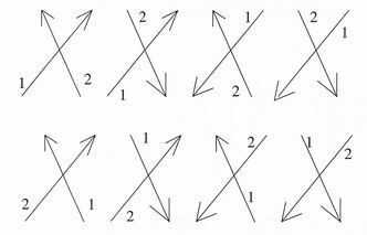
Figure 7. In a dynamic signature veryfication the timing and the order of strokes imposes limitations on the connectivity of points in the traces. A simple cross may ble drawn in 8 distinct ways.

7. Making a set of initial linkages
This is a critical step, since the problems of local minima mean that mistakes in initialisation can be computationally expensive to correct. One method is to mimic the eye by choosing in order the most distinctive features (eg local pattems or largest peak intensity) in the prototype spectrum and making the connections in this order. Alternatively only a fraction, say l/8 of the peaks, should be linked. The optimum spacing between chosen peaks would be comparable with the likely distortion. Such a selection of peaks is shown in figure 8. A search for the best linkage can then be made by examining the correlation energy only, as possible linkages are tried over the allowable range given by the existing linkages on either side. The linkage with the lowest correlation energy would be chosen. After match improving using all the energy terms, as described in the next section, a new set of links could be added between the first by doubling the number of chosen peaks, and repeating the process until all the initial connections had been made. The process of altering link positions is very much easier when only a fraction of linkages are defined, than for a full set of linkages when existing links prohibit eachother’s movements.

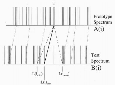
Figure 8. New links are best chosen for only a selection of possible peaks. The optimum link to the chosen peak i can initially be found from that within the allowed range with the lowest correlation energy. The selected links can then be optimised before adding more linkages.

8. Improving the match: Monte Carlo method simulated annealing
Given a set of initial linkages, even a partial one, the problem is how to reduce the total energy as far as possible. Assuming that changes in the linkages can be made only by moving links one at a time, there may need to be many intermediate unfavourable links before the best link is encountered. The total energy surface thus contains local minima which must be overcome. Monte Carlo simulated annealing is an old recipe for overcoming such problems. A "thermal energy" kT is defined and possible link changes may be accepted even when they increase the total energy. The recipe is that defined in 1952 by Metropolis et al

(i) Changes are accepted if the energy change DE due to the new linkage is less than zero DE < 0 (ii) Changes are also accepted if the energy change is such that exp(DE/kT) < rnd where rnd is a random number between 0 and l. The method eventually populates all possible states according to the Boltzmann probability function exp(-DE/kT) and so allows movements through an energy maximum towards a global energy minimum provided that the thermal energy is comparable with the barrier height. At such temperatures there is inevitably a population of non—optimal linkages. The annealing process consists of slowly reducing the thermal energy to zero so that all linkages slowly drop into their lowest energy state. The magnitude and number of tries at high themal energies must be related to the energy barriers required to be overcome.

 Copyright 1997: Colin Windsor: Last updated 4/12/2010