
Unpublished report: 1984
THE THERMAL ANNEALING OF IRRADIATED STAINLESS STEEL CONTAINING VOIDS,
C.G. WINDSOR
UKAEA, Materials Physics & Metallurgy Division, Atomic Energy Research
Establishment, Harwell, Oxon 0X11 ORA, UK
and
C.D. BRUNNING
Atomic Weapons Research Establishment, Aldermaston, Tadley, Berks, UK.
Abstract
Small angle neutron scattering (SANS) results are presented on the size distribution of voids present in a bulk specimen of irradiated stainless steel as a function of thermal annealing. The chosen sample was of FV548 and having an initial void volume fraction of 4.3%. The sample was successively annealed for 1 hour intervals at temperatures of 192, 405, 503, 601, 701, 757, 900, 998 and 1097C. The initial number weighted void diameter distribution has a bi-modal form with most probable diameters of 16 and 34 nm. Little change occurs until around 700C annealing temperature, when the size distribution broadens with more weight entering the larger voids. After annealing at 1097C the distribution changes completely with the most probable void diameter rising to around 40 nm.
1. Introduction
Under the comparatively high fast neutron irradiation doses in a fast reactor, certain materials undergo a swelling of several percent. This is caused by the formation of microscopic voids which are clearly seen in the electron microscope as roughly spherical with diameters ranging from a fraction of a nanometre to several nanometers [l]. The swelling depends on dose and irradiation temperature and so can vary across a component. This differential swelling can cause distortion of components and so makes the effect of considerable importance in the core structural and cladding materials [2]. The degree of swelling is now known to be a complicated balance between the creation of vacancies by irradiation, their mobility, their annihilation by interstitials, and their aggregation at the various possible "sinks" where voids might form [3]. At low irradiation temperatures vacancy mobility is too low for aggregation to occur, and at high temperatures vacancy annihilation by interstitials is rapid. There is therefore usually an intermediate temperature where the swelling reaches a maximum. In FV548 stainless steel the swelling maximises for irradiations around 450C.
An important question is how does an existing void distribution react to a temperature excursion, either due to a fault condition, or to a programmed annealing. Early electron microscopy by Cawthorne and Fulton [1] suggested that relatively short anneals at temperatures above 700C produced marked changes in the void size distribution. The smaller voids shrank and the larger voids grew in a process analogous to the "Ostwald" ripening of precipitates in metals [4].
The technique of small angle neutron scattering (SANS) offers the possibility of making quantitative measurements of the void size distribution non-destructively in a matter of hours or even minutes [5]. Measurements can therefore be made on the same specimen over a wide range of annealing temperatures. It is also possible to make "in situ" measurements of the size distribution changes during anealing. The SANS method uses a bulk sample several millimetres in thickness so is quite free of possible surface effects on the size distribution. There is essentially no lower size limit to the voids detectable providing they are present in quantity above a fraction of a percent in volume fraction. There is an upper limit to the diameter distribution (of a few tenths of a micron in the present experiment) caused by the instrumental resolution.
The SANS method does have some disadvantages. It measures a summation
of the effects of all defects present in the sample. In the present experiment precipitate phases will give some scattering as well as the voids. However in general voids give an exceptionally large "contrast" for small angle scattering compared to most intermetallic precipitate phases in stainless steel. The previous SANS by Windsor, Rainey and Proudfoot [6] on similar steels before annealing showed that the scattering from samples with a percent or so of void swelling much exceeded the scattering from un-irradiated heat-treated specimens. This study also showed that the volume fraction of voids estimated from SANS was in reasonable agreement with measurements made from electron microscopy and from macroscopic density changes. An important piece of evidence on the relative unimportance of precipitate scattering and the general reliability of the method is the marked reduction in the SANS scattering from cold worked, but otherwise similarly irradiated and heat-treated specimens. The amount of detectable intermetallic phases actually increases while the SANS signal decreases.
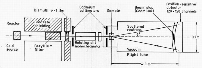
Figure 1. The layout of the Small Angle Neutron Scattering instrument at AWRE Aldermaston.
2. Experimental
Because of the likelihood that void diameters would exceed 50 nm, the experiment was performed on the SANS instrument at AWRE Aldermaston. The general layout of this spectrometer is shown in figure 1. The HERALD reactor contains a liquid hydrogen cold neutron source giving a relatively high flux of neutrons in the 0.6 to 1.2 nm wavelength range useful for SANS. Cooled beryllium and bismuth filters remove fast neutron and g ray contamination. A velocity selector provides monochromatic neutrons to within a wavelength spread Dl/l of order 14%. For this experiment a sample to detector distance of 4.3 m was chosen. Used with 0.8 nm wavelength neutrons this gives a size definition from around 47 nm down to 10 nm. At a cost of a factor of around 5 in neutron flux, 1.2 nm incident wavelength neutrons gives a range from 70 nm to 15 nm. Shorter 3h runs at 0.8 nm wavelength were therefore performed at each annealing temperature, and longer 15h runs were performed overnight at alternate annealing temperatures. For this experiment the sample was placed in an air-filled enclosure, but the flight path to the detector was evacuated. The detector used is a 128 x 128 element position-sensitive detector. With its 0.5 cm mesh size it gave a scattered resolution considerably better than the 0.5 incident collimation defined by a 4.6 cm source aperture 4.3 m before the sample.
Table 1. The annealing temperatures and SANS runs
| Date | Sample | annealing | 0.8 nm | Run | 1.2 nm | Run |
| - | - | temp time | run | duration | run | duration |
| - | - | OC mins | number | mins | number | mins |
| 10/1/83 | FV548 | - | 757 | 217 | - | - |
| 11/1/83 | - | 192 60 | 760 | 221 | 759 | 884 |
| - | - | 405 60 | 762 | 174 | - | - |
| 12/1/83 | - | 503 60 | 765 | 177 | 764 | 874 |
| - | - | 601 60 | 767 | 174 | - | - |
| 13/1/83 | - | 701 60 | 770 | 177 | 769 | 915 |
| - | - | 757 60 | 772 | 192 | - | - |
| 14/1/83 | - | 900 60 | 774 | 172 | 773 | 915 |
| - | - | 998 60 | 775 | 184 | - | - |
| - | - | 1097 60 | 777 | 318 | 776 | 1045 |
| 15/1/83 | Empty | - | 771 | 207 | 778 | 1120 |
| 16/1/83 | Water | - | 779 | 362 | 780 | 1276 |
| 19/1/83 | Cadmium | - | 781 | 1097 | 781 | 1097 |
The sample was cylindrical with a 0.5 cm diameter and 1 cm long. To avoid possible contamination of the environment around the instrument, the ageing was performed in an active fume box outside the reactor building. Figure 2 illustrates the furnace used. The sample was contained in a pyrex tube designed so that the sample could be quickly inserted into a furnace already heated to the desired annealing temperature. The furnace temperature was controlled by a thermocouple inside the pyrex tube next to the sample. For each annealing temperature the tube was left in the furnace at temperature for about 3 hours. The tube was then removed, the vacuum broken, and the sample dropped into the tube. It was then pumped out and inserted into the furnace. This operation could be performed in a couple of minutes. The annealings were performed for exactly 60 minutes. The tube was then removed from the furnace, the vacuum broken and the sample quenched in air on a metal tray. The effective ageing time at each temperature is estimated at 55 minutes. The accuracy of the temperature was of order � 10C. The sample was carried in the tray back to the instrument and then placed with tongs into the simple cadmium holder shown inset in figure 2. The 0.5 cm diameter hole in the holder backplate defines a cylindrical beam intersecting the cylindrical sample to give an effective sample thickness of 0.4 cm. Table 1 defines the annealing temperatures and runs performed at the two wavelengths. In addition runs were taken of the sample holder alone, of a 0.1 cm thick water calibration sample and of a cadmium neutron absorbing sample.
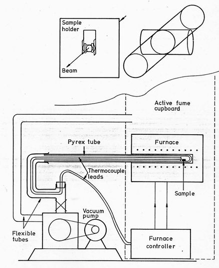
Figure 2. The furnace used for the sample annealing. The upper inset shows the sample holder, with the effective volume determined by the intersection of the 0.5 cm diameter circular beam aperture and the 0.5 cm diameter cylindrical sample.
3. The data analysis procedures
The analysis was performed using the Aldermaston suite of programs [7]. Before the main runs a short transmission run was performed with the beam stop which normally attenuates the unseattered beam removed. An analysis of this run gives the centroid of the incident beam on the counter, and also the transmission of the specimen, TS. For each run, the counter is scanned visually and noisy elements deleted from the analysis. The remaining elements are summed over circular elements of the counter, centred using the measured beam centroid with 1 cm spacing between elements. The mean counts per element IG can then be plotted against the single variable Q defined by the radial distance RG of each element, the sample to detector distance Ld and the mean wavelength l
Q = (4p/ l) sin[tan-1(Rs/Ld] (1)
The scattering vector Q is fundamental to the analysis of diffraction data. I(Q) expresses the probability of scattering from defects in the material of a size of order 2p/Q. The scattering from the sample
Is is compared with the known scattering from a standard sample of
water 1 mm thick. The effective cross-section of 1 cm3 of water at 0.8 nm wavelength for scattering
into one steradian is 0.327 cm3. This defines its macroscopic cross-section
(dp/dW)W in cm-1 steradian . By comparing the measured sample intensity Is
with that for water IW the macroscopic cross-section of the sample
(dp/dW)S
can be determined. In the proper analysis correction must also be made for several further factors. From all intensities we have first to subtract the signal independent detector background ICd as measured with a cadmium sample. From the sample and water intensities we must also subtract a
background intensity IBg. However this must be attenuated by the sample
g or water transmission T to allow for the reduction in the component of
background proportional to the neutrons in the beam. Similarly the sample scattering must be divided by the transmission to give the cross-section which would have been measured in the absence of attenuation of the beam. The macroscopic cross-section must also be weighted by the respective thickness t of the sample and water runs. All measured intensities I must be normalised by the run duration D. Using suffixes S, Cd, W and Bg to represent sample, cadmium, water and background runs respectively, the expression used for evaluating the macroscopic cross-section is
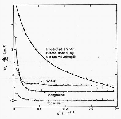
Figure 3. The SANS data for the unirradiated specimen compared with the background, cadmium and water calibration runs. The data are plotted as Guinier plots normalised to the sample macroscopic cross-section.
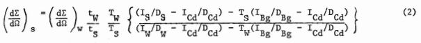
Figure 3 shows a plot of the four individual component spectra processed as an effective sample macroscopic cross-section. The sample was the unannealed steel measured at 0.8 nm wavelength. The signal to background ratio is greater than 2 up to Q values of order 0.5 nm . The peak in the background and cadmium runs at low Q values is not a serious correction.
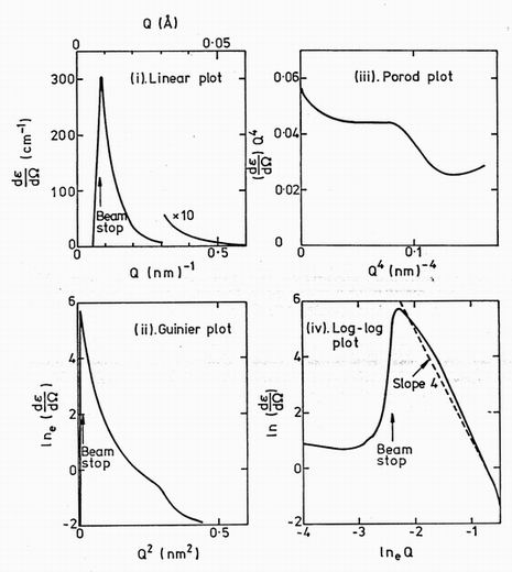
Figure 4. Alternative plots of the macroscopic cross-section (dp/dW)W for irradiated PV548 before annealing.
4. Presentation and analysis of the results
The macroscopic cross-section given by equation 2 can be presented in various ways to bring out different features of the scattering 5 Four of these are illustrated in figure 4.
(i) The linear plot. The scattering is very strongly peaked at low angles or low Q vectors making a linear plot of cross-section against Q value not very informative. The beam stop position represents a limit of useful data.
(ii) The Guinier plot. This graph of lne(dp/dW)W against Q will be used in most of the subsequent figures. This plot is particularly easy to interpret since a set of roughly spherical voids of diameter D matrix scattering length density p and volume fraction c gives rise to the linear Guinier plot expressed in the cross-section
(dS/d This equation is only valid for values of the product QD less than about 6. At higher values the exponential law breaks down progressively, and the Guinier plot becomes curved. The Guinier plot of figure 4(ii) is curved over all its range showing that the assumption of a single void diameter is not valid. There is instead a broad distribution of void diameters. This can be analysed into a diameter distribution as described in paragraph 9.
(iii) The Porod plot. At values of the product QD greater than 12 or so, the scattering cross-section from a void system of specific surface area S per unit volume approaches
(dS/d Thus a Porod plot of
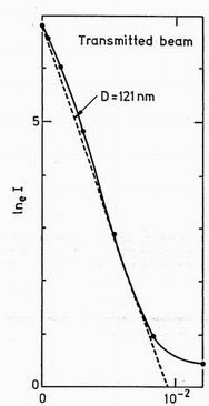
QdS/d Figure 5. A Guinier plot ot the transmitted beam showing its broadening due to instrumental resolution.
The slope corresponds to voids of 121 nm diameter.
5. The effects of instrumental resolution
The upper limit to the void sizes visible in this study is dependent on the instrumental resolution, in particular on the breadth of the signal seen at the counter in the absence of sample scattering. Figure 5 shows a Guinier plot of this intensity with 0.8 nm neutrons. The plot is linear suggesting a Gaussian intensity distribution. Its slope corresponds to scattering from particles of diameter 121.2 nm. This represents an upper limit to observable voids and diameters over say 80 nm will be imperfectly visible. At 1.2 nm wavelength these sizes increase by 50%. No correction for resolution will be made in this paper, apart from the data in figure 9.
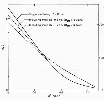
Figure 6. Guinier plots of (i) the calculated single scattering for 17 nm diameter
spheres with 4.8% volume fraction (solid line); (ii) The scattering including multiple
scattering at 0.8 nm wavelength. The slope of the linear region below Q2 =0.1 nm-1
gives the effective diameter shown, (iii) The effect of multiple scattering at 1.2 nm wavelength.
6. The effects of multiple scattering
The usual assumption of SANS is that the cross-section is small enough that the scattering probability is relatively low so that multiple scattering is negligible. This sample, with its intense void scattering, actually scattered some 47.4% of the 0.8 nm beam and 75.6% of the 1.2 nm beam. Multiple scattering could not therefore be neglected. An estimate was made using the program of Brunning [8] which is based on the theory described by Schelten and Schmatz [9]. The program assumes a mean void diameter, and figure 6 illustrates the magnitude of the effect for a void diameter distribution centred on 17 nm and with 4.8% voids volume fraction which gives the observed transmission of 0.53 at 0.8 nm wavelength. Including the multiple scattering at 0.8 nm reproduces a linear plot but corresponding to a 5% reduction in the void diameter. The intensity at Q = 0 giving the Guinier constant is reduced by some 37%, while the Porod region scattering increases and spoils the Porod law. At 1.2 nm wavelength the Guinier diameter is 14% too low and the Guinier constant reduced by 62%. Thus multiple scattering will clearly give size errors in our results of some 10%
and volume fraction errors of order 50%. Since a multiple scattering correction is not at present possible for a general diameter distribution no correction has been made in the subsequent data.
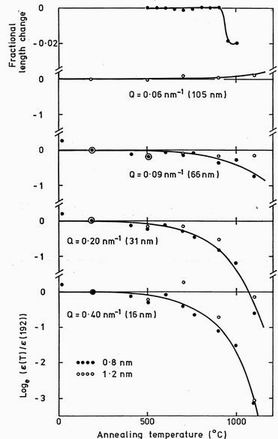
Figure 7. The changes in SANS macroscopic cross-section as a function of the temperature reached in the cumulative annealing. The upper curve shows the length measurements of Watkin [10].
7. Relative scattering changes during annealing
Before attempting to define the absolute scattering cross-section we show in figure 7 the relative changes in the scattering cross-section
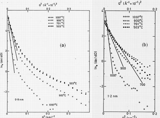
dS/d Figure 8. Guinier plot of the macroscopic cross-section showing the change in void population with the annealing temperature reached. The results are measured with
(a) on the left, 0.8 nm neutrons and not corrected for resolution or multiple scattering. (b) on the right, is for
1.2 nm wavelength.
8. The macroscopic cross-section results
Figures 8a and 8b show the macroscopic cross-section calculated using equation 2 without further corrections. To improve the statistical accuracy the water calibration term in the denominator was smoothed by hand. Only the results at 500, 700, 900 and 1100C annealing temperatures are shown.
Results at temperatures up to 700C show only a scatter commensurate with the error of a few percent inherent in removing and replacing the sample. At 900C annealing the cross-section is reduced at bigger Q values and rises more steeply at low Q indicating an increase in the mean size of the scattering centres. At 1097C annealing the rise at low Q increases indicating the formation of yet larger voids.
The agreement between the 0.8 and 1.2 nm results is good only at the
lowest scattering intensities below e-2 . At higher intensities the results
diverge in the directions suggested by our multiple scattering correction of figure 6. The longer wavelength results have the smaller slope and lower intensity suggested by the calculations. A quantitative correction cannot be made due to the presence of a significant size distribution.
The Porod plot of figure 4(iii) suggests that the Q range 0.4 to 0.6 nm-1
(Q2 = 0.15 to 0.3 nm-2) is satisfying the Porod law
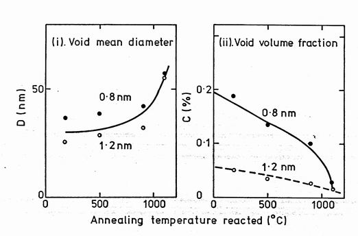
Q4dS/d Figure 9. Figure 9. The mean void diameter D and volume fraction C deduced from the linear region of the Guinier plots of figures 8a and 8b. The points and open circles represent 0.8 and 1.2 nm results respectively. The lines above the diameter points show the effect of the resolution correction of equation 5.
The lower limit of points in figure 9(ii) show the
mean diameter calculated from the slopes of the lines in figure 8. The upper limit shows the effect of resolution allowing for the resolution Dres = 181.2 at 1.2 nm using the expression
Dcorr-2 = Dobs-2
- Dres-2 (5)
The resolution correction is only significant at 0.8 nm for the highest temperature. The two wavelengths give a reasonable agreement in diameter considering the likely effect of multiple scattering. The volume fraction deduced from the intercept of the Guinier line at Q = 0 is plotted in figure 9(ii). The 0.8 nm-1 results reduce steadily from 0.2% void fraction to a very small value at 1100C. The 1.2 nm results are smaller by a factor of 4. We feel multiple scattering is probably responsible for this discrepancy. The correction is still large at 0.8 nm and we feel the volume fraction results should not be used except with caution.
Figure 10. The volume-weighted size distribution of voids measured (i) At 0.6 nm using the Harwell SANS instrument (smooth line) (ii) At 0.8 nm using Herald SA1 (dotted) (iii) At 1.2 nm (dashed). The different Q ranges covered lead to
different spatial ranges covered.
9. The void diameter distribution function
The generally curved Guinier plots observed in figure 8 suggests that the assumption of a single mean void size is not valid. The diameter distribution can be expressed directly using programs such as that by Vonk [11] which use least squares methods to find a histogram of diameters which reproduces the observed Q dependence of the scattering. There are several difficulties in these methods. Firstly as assumption of the shape of the voids must be made. Spherical voids have been assumed in our calculations. Secondly data should ideally exist over the whole range of Q from zero to infinity. Our data of limited range needs to be extrapolated by using a Guinier fit at low Q values. The high Q truncation causes termination ripples in the distribution. In the Vonk method these can actually give rise to unphysical negative regions of the distribution. That there must be reservations on the results from Vonk's program is illustrated by figure 10 where we superimpose the diameter distribution for the unirradiated sample (i) measured previously on the Harwell SANS at 0.6 nm wavelength (ii) measured at 0.8 nm wavelength in this experiment and (iii) measured at 1.2 nm (and at 192C annealing) in this experiment. The much larger Q range of the Harwell results reveal a strong distribution at 2.5 nm diameter but give poor resolution at larger diameters. The 0.8 nm results give a double-peaked distribution but again lack resolution at the higher sizes. The 1.2 nm results give a similar double-peaked distribution but slightly displaced to higher sizes and with more weight in the smaller diameter. The 1.2 nm results have the best resolution for the larger pores of interest in the annealing so we give most weight to the 1.2 nm results.
Figure 11. The volume weighted size distribution of voids in FV 548 stainless steel irradiated to 34 dpa at 461C. The data are from small angle scattering using 1.2 nm neutrons transformed using the VONK program. A single specimen was progressively annealed for one hour at roughly 100C intervals up to the temperature shown.
Figure 11 shows the change in size distribution during the annealing experiment. The distribution shows very little change up to 700C with most probable diameters at 16 and 34 nm. However at 900C annealing the double-peaked distribution moves into a broader distribution extending to some 60 nm. At 1097C annealing the distribution changes completely with the most probable void diameter increasing to around 40 nm.
10. Discussion
Small angle neutron scattering is very sensitive to void size distributions in the size range from 2 to 50 nm diameter. This is caused by the high
scattering length contrast of voids with the matrix compared with say intermetallic precipitates, and by their high volume fraction of a few percent. The technique applied to the FV548 specimen "LOG" showed only small changes during successive annealings of one hour up to 700C. At higher temperatures the scattering distribution changes increasingly rapidly. However the changes are continuous in contrast to the sharp change seen in specimen dimensions. The direction of the changes follows the pattern expected from microscopy of a change from a high volume fraction of small voids to a smaller fraction of larger voids. Quantitatively the measurements suggest an increase in the mean void diameter from around 20 nm before annealing to around 50 nm after annealing at 1097C. The quantitative analysis is complicated by the strength of the scattering which led to strong multiple scattering. This is difficult to correct for at this stage. In retrospect a thin 0.5 mm specimen would have given much more precise data with adequate statistics.
References
1 C Cawthorne and E J Fulton. Nature 216 (1967) 575.


2 Harries
3 A D Brailsford and R Bullough. J Nucl Mat 44 (1972) 121-135.
4 J W Christian "The Theory of Transformations in Metals and Alloys"
2nd Ed Pergamon Press, Oxford 1975.
5 "Treatise on Materials Science and Technology" Vol 15, Neutron Scattering,
Ed G Kostorz, Academic Press, New York 1979.
6 C G Windsor, G Proudfoot and V S Rainey. To be published.
7 R J Barton. Unpublished Report AWRE Aldermaston NP 81/
8 CD Brunning. Unpublished Report AWRE Aldermaston NP 81/5.
9 J Schelten and W Sehmatz. J Appl Cryst 13(1980) 385.
10 J Watkin (Private communication).
11 C G Vonk J Appl Cryst 9 (1976) 433.