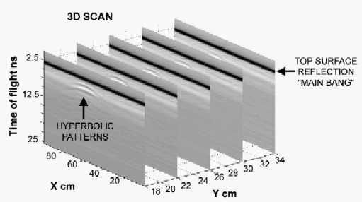
Figure 2: An example of the reflected amplitude (grey scale) as a function of range (time of flight) and position along the scan (X) for several parallel scans (Y).
Keywords: signal processing, ground penetrating radar, landmines, buried objects, classification
Buried Mine Classification from three-dimensional RADAR data
Lorenzo Capineri*, PierLuigi Falorni* C. G. Windsor+
* Dipartimento Elettronica e Telecomunicazioni, Universita degli Studi di Firenze, Via S. Marta 3, 50139 Firenze, Italy, Tel/Fax +39 055 4796376/517, Capineri@ieee.org, Pfalorni@supereva.it
116, New Road, East Hagbourne, OX11 9LD, Tel +44 01235 812083 colin.windsor@virgin.net
Abstract:
Ground penetrating RADAR has become an important tool in anti-personnel mine detection. In general a buried object can be detected by scanning the ground surface with the radar probe. An object whose size is comparable with a typical wavelength (0.1m @ 1 GHz) gives rise to a complex reflection pattern consisting of a superposition of inverted hyperbolic arcs in three dimensions (3-D). Previous papers have described the codes which use the gradient information in the scattering data to replace each overlapping arc by an "apex point" describing the 3-D position, amplitude and sign of each arc. This paper introduces the concept of a "pendant": a series of reflections whose apexes lie close to a vertical column which may be identified as arising from a single object. The amplitudes of these reflections may be used a features for object classification. The method is demonstrated using radar images from a buried isolated mine and also in proximity with other objects. The aim of this classification scheme is the identification of one object (mine) type against more "point-like" signals from "clutter" objects small compared to the wavelength.
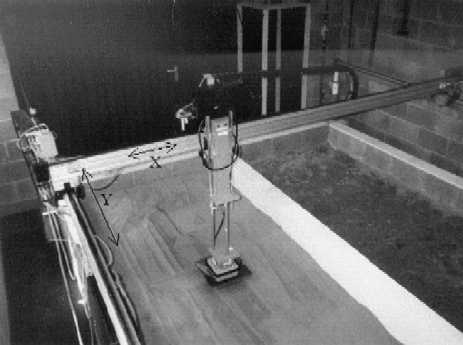
Figure 1: The earth box containing buried mines and other objects at the LAMI-DETEC laboratory in Lausanne used to collect the data presented here.
1. Introduction
A scanned ground penetrating
RADAR beam gives rise to a complex 3-D pattern of scattered intensity when
reflected by a buried object. While there has been much work on the detection
and location of buried objects (1)(2)(3), it would be highly
desirable to be able to distinguish the mines from the welter of other benign
buried objects that can give a significant reflected intensity. A problem is
that human interpretation is difficult because of the large quantity of
information that needs to be displayed. This classification problem has been
already tacled with several techniques by other authors (4)(5)(6).
For example a mine buried 10 cm deep in sand and scanned using a 2 cm raster
may show signals over 20 cm in both directions. Neither a single plot of range
along a scan (B-scan) nor signal amplitude at a given range (C-scan) provide
more than a fraction of the useful information available in 3-D.
Classification is possible because of the
relatively large size of most mines compared to the wavelength, and compared to
the size of many other strongly reflecting objects. The incident RADAR pulse
usually contains a wavelet with only a couple of maxima, but the reflected
pulse from a mine is composed of a superposition of reflections from the
various mine interfaces, including some multiple reflections, and is likely to
contain at several maxima whose relative intensities are characteristic of the
particular mine.
Figure 2: An example of the reflected amplitude
(grey scale) as a function of range (time of flight) and position along the scan
(X) for several parallel scans (Y).
Figure 1 shows how the data used in this paper were obtained at the LAMI-DETEC institute(7). The 1 GHz source was scanned over a box 1.5 m deep and filled with sand or earth. Typical values for the central wavelength at 1 GHz in an average soil is 10 cm. Various objects were placed in the box at known positions and depths. Raster scans were performed with the reflected intensity as a function of time, being recorded along a 1 m long path along the X-direction. The position of the antenna in contact with the ground was then stepped by 2 cm in the Y direction, perpendicular to the original scan. In this way a series of acquisitions along parallel planes are devised and this form a 3-D data set, as shown in Figure 2.
An example of typical B-scan containing reflections from a mine buried in sand is also shown in figure 2. The strong black flat reflection at the top is the "main bang" indicating the reflection from the surface of the sand. Its range can be used to calibrate the depth. The mine shows up as a series of inverted hyperbolic arcs, whose apex defines the lateral position of the mine along the scan, and whose range defines both the depth and the vertical extent of the mine. Regarding the alternation of the signal maxima and minima, Figure 3 illustrates the way the composite signal shown in figure 2 at each probe position, might be constructed from the various planar interfaces of the mine and perpendicular to the probe vertical axis. Reflections from the upper and lower surfaces occur with various defined amplitudes and phases according to the dielectric properties of the materials. In addition there may be significant multiple reflections. The summation of all these signals gives rise to a complex waveform containing several "ripples". The separation of the peaks is roughly constant being determined by the wavelength. Their amplitude and phase is characteristic of the structure of the mine(8). A small but strongly scattering object, such a piece of scrapnel a few centimetres across, gives a reflected signal whose profile is much more like the incident wave, and so is easily distinguished.
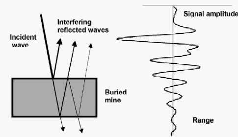
Figure 3. Each interface in the mine partially reflects and partially transmits the incident wave. The reflected waves constructively interfere and generate a broadened wavelet whose profile is characteristic of the construction of the mine
2. The location of hyperbolic arcs and their apex points
The new approach pursued in this work for the classification of buried object is the notion of tridimensional contrast pattern derived from the acquisition of 3-D data. This contrast pattern is generated in the most simple case of a point-like object buried at position (x0,y0, z0), by the amplitudes of the scattered signals at different times of flight (TOF) gathered at surface positions (x,y, 0) with a Radar probe:
TOF= 2*[(x-x0)2 +(y-y0)2 +zo2]1/2/Vwhere V is the propagation velocity of the medium.
The range can be easily derived from the previous TOF equation by assuming V constant, which is true for a homogeneous medium. The contrast patterns appear as stacked hyperbolic functions in the x,y,TOF representation due to the alternations of positive and negative peaks of the scattered signals. The proposed algorithm is aimed to extract the hyperbolic contrast patterns from the 3-D data set that will be used to retrieve essential buried object characteristics from their spatial position, morphology and phase information. The exploitation of this concept will be described in the next sections. However this task is not trivial considering the following experimental conditions:
1. Limited spatial and bandwidth of the Radar
2. Poor approximation of point-like object
3. Clutter (surrounding debris)
4. Inhomogeneous medium
Regarding the difficult problem of clutter reduction we decided to design an algorithm composed of several successive steps in order to reduce progressively the problem complexity and to enhance the object characteristic response. The problem of automatic hyperbolic arc extraction has been studied for two-dimensional images and the results obtained with different techniques on simulated and real images have been published.(3)(9)(10)
The processing scheme applied to the available data starts with the background removal, which consists in the application of a standard linear high-pass filter along the scanning direction. The typical effect is the cancellation from the image of the high level pulse reflected at the air to ground interface which increases the grey levels dynamic for the useful signals (see example in Figure 2). The second processing step is the gradient calculation to define the image contrast. The hyperbolic patterns are originated from ringing signals and they can be precisely defined by calculating the vector gradient using the intensity level f(x,y,z=const) Local properties of the 3-D image f(x,y,z) are retained and the morphological information of the buried object response are estimated by the 3-D gradient. We found this approach more robust than other methods based on signal amplitudes. The image contrast is defined by the 3-D gradient
Df(x,y,z)=(df/dx,df/dy,df/dz).
The partial derivatives have been calculated using the central finite differences method. The calculation of the gradient over a mesh provides a vector field that can be used to estimate the flux lines. The flux lines describe the ridges of the hyperbolic patterns that can be calculated by exploiting the change in the sign of the gradient corresponding to local maximum or minimum. For example the change of the gradient sign can be determined by the convolution of the gradient with a function QT defined as:
GS[f(t)] = sign[f'(t) x QT(t) where QT(t) = 1 if t betweem 0 and T/2
= -1 of t between -T/2 and 0 and = 0 elsewhere
where T is the period corresponding to the Radar pulse central frequency and t is a parameter that indicate a position along a flux line.
For a better understanding of how a typical contrast pattern looks like, Figure 4 shows the first three contrast patterns found on a PFM mine scan: the first and the third pattern are obtained by the negative phase waves and the second one with the positive phase waves.
�������������������������������������������������������������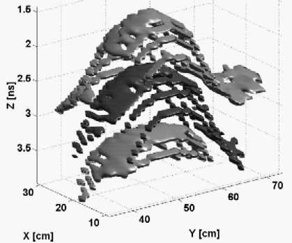
Figure 4: An example of first three contrast patterns extracted with gradient-sigmoid filter from data of a PFM mine buried at 10 cm in sand (dark gray positive phase, light gray negative phase) plotted in the X,Y and range (time of flight) coordinate system..
The next step is the classification of these patterns by assigning to the points belonging to the same pattern a code number and an associated colour. A colour bar with number codes will be printed together with the final visualization of results for object identification. Finally for data reduction only the set of points with cardinality higher than a predefined threshold are stored.
The final processing before the visualization is the transformation of extracted
points from the variable space (x,y,TOF) into real space hyperboloid centres
(x0,y0,z0)
defining a buried object position. This process employs a modified version of
the Random Hough Transform(11) which selects randomly triplets of
points {(xi,yi,TOFi), i=1,2,3} within the same pattern and inverts the distance function di=
TOFi V /2 . The transformation solves a system of 3 equations with
three unknowns (x0,y0,z0) and it calculates a
possible hyperboloid position. This position is accumulated and the inversion
process repeated many times until all the points of the patterns are
considered. The same process is applied for all extracted patterns. Each
estimated position is affected by an error due to the uncertainty of the
measurements (Ex, Ey, ETOF); this means that
all the accumulated positions are scattered around the nominal object position
(x0,y0,z0), according to the equivalence
between depth (z) and time of flight (TOF). Then patterns with many points that
are well correlated with a hyperboloid function provide high scores and low
variance. Their representation in 3-D is a sphere having a radius proportional
to the score and three segments proportional to the variances
(
The above method has been tested also with some extended objects (size comparable to few wavelengths) and it has been assumed an object scattering model consisting of a distribution of point-like scatterers on the object surface. In particular it has been also verified that contours of sharp objects can also be detected because their points give rise to a hyperbolic-like functions. A mathematical model is under study to consider the relative contrast patterns as an extension of the objects contours according to the hyperbolic transformation provided by the above equation for TOF.
3. The sorting of apex points into "pendants"
The apex points located during scan over a mine will generally look as in figure 5. The mine itself, being relatively large in the scale of the wavelength, will generally give a series of apexes of opposite sign extending downwards in depth. The smaller "debris" objects will generally be described by just one or two apexes, while larger benign objects such as a coke bottle, may again show several apexes.
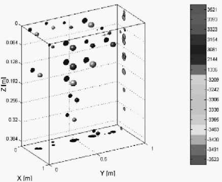
Figure 5: The apex points determined from the scans over a PMN mine buried at 5 cm depth in earth. The colour coded spheres indicate the positions of the apexes. All spheres are projected on the xy, yz, zx planes. On the right the palette shows the map of set's code versus sphere colour..
The set of apex points generated from the reflections from a single buried object will generally satisfy all of the following conditions.
1. They fall into a vertical column above each other within a specified distance tolerance Dx=Dy of say 0.06 m
2. The vertical spacing between points should fall, within a specified tolerance Dz, of a constant distance equal to half the wavelength l within the medium. Typically Dz is say 0.015 m for a wavelength of around 0.1 m
3. "White" high phase apex points must alternate with "black" low phase points
The phase of each part of the reflection is a key variable in its use for pendant location. Since the main bang in this series of measurements was "white", the extraction was started by searching for the most intense white apex point within the image. If the weight of this reflection lay above a specified threshold, the point was confirmed as the start of a potential pendant series. A search over all "black" points in the image was then made, at deeper depths for points present within the allowed volume defined by the current values of Dx, Dy, Dz and l. These volumes are denoted by the small rectangles in figure 6. The optimal value of l was later refined by evaluating a running total of the accepted vertical spacings. Generally only one point in the image satisfied the criteria. However in case more than one point was within the allowed volume, the one whose distance was closest to the predicted position was taken. If at least one point was found the extraction continued, but with the phase of the search changed to look for the next deeper white point. If no point was found within the currently specified volume, the search still deeper was abandoned. The extraction then continued from the original most intense point, but to more shallow depths. The volume definition parameters used were Dx=0.015m, Dy=0.015m, Dz=0.015m and l/2=0.045m.
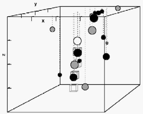
Figure 6: The apex points determined from the scans over a PMN mine buried at 5cm depth in earth. The four spheres joined by a line represent the pendant created by the mine. The boxes show the volume in real space where a search for a successful new apex of the correct sign was made.
Many of the noise reflections gave only a single point in the pendant series, corresponding to an object small compared to the wavelength. However several of the reflections gave rise to a series of up to 5 apex points of alternating sign. The weights of each point of the series have been divided by their average weight so that the patterns are unaffected by absolute changes in contrast. The first white point is generally the largest, and is often preceded by a single black point and followed by a black, a white, and sometimes a further black point. Five feature parameters were therefore chosen for classification in this study. They were the weights of the leading black, principal white, next black, next white and next black, divided by their average weight.
4. The training and test data used to classify mines from other objects
The data at our disposal consisted of scans over PMN mines at varying depths in sand and in earth, and a test scan containing a PMA mine, a metal ring and a bottle, all giving relatively intense signals compared with the noise level.The two mimicking landmines used in the laboratory(7) are very similar and they have the following characteristics: PMA-3 cylindrical mine with diameter 10 mm, height 50 mm, RTV filled; PMN diameter 112 mm, height 56 mm. PMN mine half filled with the replacing silicon. There were four scans over sand, with a PMN mine at depth 1, 3, 5, and 10 cm. In these cases the PMN mine being the only significant object in each scan and all gave clear pendants. The three scans over earth had the mine at 3, 5 and 10cm depth. The mine signal was always clear but in earth it was together with other several smaller signals that could also be classified as noise objects. All the mines gave good pendants similar to that in figure 6. These 7 scans over mines formed the basis of the training data. The quality of the data can be seen from the first seven (solid line) traces in figure 7 which show the five normalised feature parameters for the mine pendants at different depths in sand and earth.
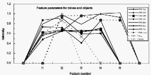
Figure 7: The feature parameter amplitudes for the training and test scans. The training data ( full lines) are all for PMN mines at varying depths in sand and earth. The test data (dashed lines) covers an area of earth containing a mine a metal ring and a bottle
The test data consisted of a set of scans over an earth tray containing several objects. One was a PMA mine, one a ring of metal, and one a bottle. All these objects gave strong signal, and there were in addition several smaller signals from stones and other objects present in the earth. Figure 8 shows a perspective view, as in figure 5, of the apex points recorded over this area. Again the diameter of the circles represents the amplitude of the feature, and the grey and black colours the positive and negative phases. A pendant with 4 features is seen from the mine, the metal ring has only 3 features and the bottle only one.
A surface view over the area of figure 8 is shown in figure 9. This
representation makes clear how close to the vertical are the apexes of the
reflections from the objects. In fact the separation of the three objects is
shown to be much better than might have been estimated from the perspective
plot of figure 8.
Figure 8: A three-dimensional view of the apex points determined
from� scans over an area of earth
containing known objects, a PMA mine, a ,metal ring and a bottle. X and Y
represent the position over the ground and Z the depth. 5. The classification of mines from other buried
objects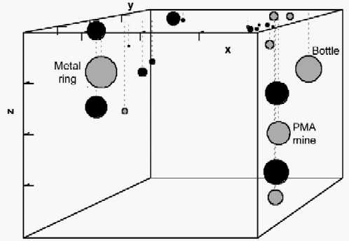
Both the conventional Kth nearest neighbour and neural network MLP classifiers have been applied to this problem. Neural networks act as non-linear mappings which are able to use the 5-dimensional feature space input to find the optimal classification from training data.
The Multi-Layer
Perceptron (MLP) network is widely used and has the structure shown in figure
10 (12). The n0=5
feature parameters a0i, i=1, n0
are inputs to the nh
"neurons" in the "hidden" layer. These neurons j=1,nh take a linear combination of the inputs, multiply
them by adjustable hidden unit weights wijh,
subtract an offset w0jh, and evaluate a sigmoidal function s(x) in order to
define the next layer outputs a1j = s(Si=1,n0 ��a0iwijh
w0jh), where s(x)=1/(1+e-x). This sigmoid function gives 0
for x large, 0.5 for x=1 and 1 for x very small. The second "target" layer has similarly takes, for
each target neuron k, the results
from the j=1,nh hidden
units multiplied them by a further set of target weights wikt with an offset w0kt.2k = s(Sk=1,nh ��a1jjkjk2 w0k2).
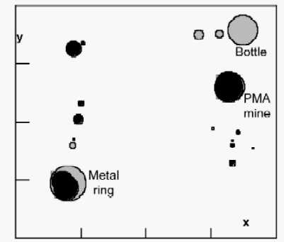
Figure 9: The apex points determined from scans over an area of earth containing known objects, a PMA mine, a ,metal ring and a bottle
Training involves minimising the residual R between the targets tk(e) and the outputs a2k(e) for each example eR =�� S k=1,n2 �(tk(e) � a2k(e))2
Weights wij are adjusted according to
Dwji =
hd2j a1k� ������������ where� d2j �= S j=1,n2� (tj � a2j) a2j (
1 - �a2j) and h is a factor for adjusting the
learning rate.
During
the training process the two sets of weights are adjusted until the
least-squares residual between the targets tk(e), for the eth
example object and the kth
target and the network output a2k,
are a minimum. The number of hidden units is crucial. If it is too small the
network has insufficient complexity to fit the training data. If it is too
large, a common problem with larger networks, then the network "over-fits" and
fails to fit the test data(13).
As might be guessed from the features of figure 7, this problem of classifying the dashed objects proved straightforward for either the Kth nearest neighbour and neural network MLP classifiers. Using a single target for the mine, and classifying all other objects as noise, gave no errors using either classifier.
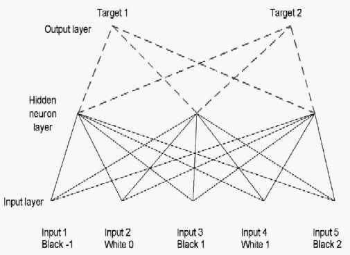
Figure 10: The structure of a Multi-Layer Perceptron neural network used in this work. A weighted sum over the 5 input signals is converted by each "neuron" into an output signal which is sent to the succeeding layer of two "output" neurons, one for each class of specific object.
6. Results of the classification of buried test objects
In this work a method for the estimation of buried objects response by using 3-D
contrast patterns has been developed. A new "pendant" concept has been
introduced to obtain a simple feature set for classification with standard
classifiers. We found also that the visualisation of pendants provides a more
easily intelligible picture for the user. According to this method a
consistent feature sets for shallow (1 cm) and deeper (10 cm) PMN mines in sand and soil have been calculated and preliminary results on the classification process has been successful for a one mine type classification in different ground conditions. Future developments of this work in progress will be addressed to the classification and visualisation of other 3-D sets containing both mines and other objects.
Acknowledgements
Prof. Leonardo Masotti has made this work possible with grants from the University of Florence for short-term mobility, and from the Italian CNR. We also acknowledge the contribution of Giuseppe Davoli for insights on the nature of interference in reflections from complex objects.
6. References
1.. RUMELHART D. E. et al.Learning internal representions by error propagation, Parallel distributed processing. MIT Press, Cambridge. MA, 1986.
2. CROALL. I. F. and MASON J. P. (eds) Industrial applications of neural networks. Springer Verlag. 1991.
3. WINDSOR C. G. et al. The classification of defects from ultrasonic images: a neural network approach. Brit. J. NDT; 1993, 5, 15-22.
4. MASON I. P. et al. A novel algorithm for chromatogram matching in qualitative analysis. J. High Res. Chromatag., 1992, 15. 539-547,5. O'BRIAN M. and ROBINSON D. Setting the course for a commercial power plant, ATOM, 1994, 434, 32-35.
6. BISHOP C M. et al. Hardware implementation of a neural network to control plasma position in COMPASS-D. Fusion Technol., 1993, 997-1001.
Authors biographies
Lorenzo Capineri received the Laurea in Electronic Engineering in 1988, and the Doctorate in Non Destructive Testing in 1993. Since 1995 he has been associate researcher in Electronics at the Department of Electronic Engineering of the University of Florence, Italy. His current research activities are in design of ultrasonic and pyroelectric sensors, electronic instruments design and ultrasound signal processing for Non Destructive Testing and Biomedical applications. Since 1991 he has collaborated with AEA Technology, Harwell Laboratory UK, in the field of ultrasonic and ground penetrating radar signal processing. Home page: www.echommunity.com/staff.htm
PierLuigi Falorni graduated in Informatic Engineering with Laurea degree at Universita degli Studi di Firenze with a thesis on advanced processing methods for ground penetrating data (GPR). At present he is doctorate student in Non Destructive Testing at the same University, and he is coauthor of two papers on GPR image processing. He presented an invited paper at the international conference PIERS 2002 in Boston. He collaborates with company IDS S.p.A. in Pisa (Italy) and he is a consultant in informatics of several important italian companies.
Colin G. Windsor: Dr Colin G Windsor FRS, DPhil, FInstP, FInstNDT, 116, New Road, East Hagbourne, OX11 9LD, UK ,Colin Windsor read Physics at Oxford, followed by a DPhil measuring magnetic materials and a PostDoc year at Yale. He returned to Harwell in its golden years to study itinerant metals using neutron scattering and simulation. He later used neural networks in a variety of industrial applications particularly signature verification. He is now a consultant with UKAEA fusion. Home page: www.freespace.virgin.net/colin.windsor.