A Data Pair-Labeled Generalized Hough Transform for Radar Location of Buried Objects

C.G. Windsor^a, L. Capineri^b, P. Falorni^b

^a116, New Road, East Hagbourne, OX11 9LD, UK

^bDept of Electronics and Telecommunications, University of Florence, Via S. Marta 3, 50139, Florence, Italy

Abstract A method is presented for isolating the overlapping hyperbolic arcs found when a radar scan is made over several adjacent buried objects. The reflected signal is first converted into a series of data pairs (y_j, t_j) giving, for a radar antennae position y_j along the scan, the times-of-flight t_j of the maxima or minima in the reflected radar amplitude. The generalised Hough transform method has been extended to record in an associative store the sets of data pairs contributing to each bin in the Hough accumulator space. A cluster of high bins, defining a peak in this space, may then be broken down into its contributing data pairs. This gives the important advantage that conventional least squares algorithm can be used to reveal the object position, depth, and radius or velocity. The method is demonstrated on real radar data from buried pipes. The radius of a 0.18m radius concrete pipe at 1m depth is estimated at 0.14m.

Keywords: Ground-penetrating radar, Generalised Hough transform, buried pipes, diameter measurement

I. INTRODUCTION

THE LOCATION of buried targets from ground penetrating radar data is a common problem for nondestructive evaluation of civil structures [1], concrete [2], soil [3], archaeology [4], and for landmine detection [5]. Here, we present a method that is able to isolate the radar reflection from a particular buried object. For example, in surface scans perpendicular to several buried pipes, each buried pipe gives a wavelet of reflections, forming inverted hyperbolic arcs that may overlap to give a complex pattern. Human eyes are generally good at separating these arcs, but automatic characterization is not easy. Mathematically, to determine the real space positions of the pipes from the reflected radar pattern is an inverse problem of some complexity. Standard treatments include synthetic aperture focussing [6], frequency domain field inversion [6], genetic algorithms [7], and neural networks [8].

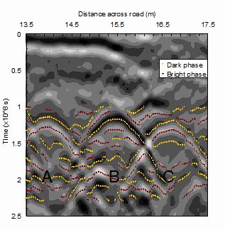
Fig. 1. Reflected radar intensity (grayscale) as the radar probe is scanned` across a road as a function of the position (Y_i) and the time-of-flight (t_i). The dark circles are the bright (positive) phase maxima and the light circles the dark phase (negative) minima. The three objects A,B, and C are utilities buried in the road.

The Hough transform originated in image analysis [9] with two variables. The extended Hough transform using more variablesfs was used in radar time of flight in [10], and extended to pipes of finite diameter in [11]-[14]. In a recent comprehensive analysis [15], the general case of pipes at a given position Y , depth Z, radius R, measured in a medium of unknown velocity V , was considered.

II. EXPERIMENTAL ARRANGEMENT FOR RADAR DETECTION OF BURIED OBJECTS

A radar antenna, placed just above the surface, is scanned across the objects to give a B-scan, defining the reflected intensity S(y, t) as a function of the round-trip time of flight t along the scan Y . Each buried object gives a generally hyperbolic pattern as the range becomes a minimum when the antenna is over the object, as shown in Fig. 1. This shows the conventional B-scan representation of the reflected intensity as a grey scale, representing reflected intensity, with time of flight t vertical, and distance Y across the road horizontal. The source was a FC = 600 MHz central frequency pulsed RIS model radar developed by the IDS company in Pisa, Italy [16]. The image is acquired with a time sampling of TS = 2.5 x 10^-8s, and with a lateral step of 0.01 m. The average soil velocity V was estimated at 1.23 x 10⁸ ms^-1 and so the wavelength lC = V/FC = 0.205m and the time sampling TS corresponds to a distance V.TS/2 = 0.0154m. The problem is that in general there are many overlapping signals from the different buried objects, and many spurious signals arising from extraneous objects, such as stones, and from layered structures in the ground. The location was a test ground, and the nature of some objects was known. The inverted hyperbola in the center (denoted by B in Fig. 1) is known to be from a concrete pipe 0.36m in diameter, buried at a depth of about 1m. The reflection on the right-hand side, (C), is from an electric utility cable of 0.08-m diameter. The nature of the strong reflection to the left (A) is unknown. The different nature of the reflecting objects is shown by the phase of the principal reflected signal. The concrete pipe gives a dark-phase principal reflection with ringing satellite arcs above and below. The other two objects have a light-phase principal reflection with weaker satellites. The problem faced is clear. The reflections from the three main objects overlap to a considerable degree. Also there is considerable clutter noise from the nature of the soil, and to the top of the figure, rather intense flat signals representing the layered structure of the road. Presented here is an automatic method for isolating the reflected signals from any one object.

III. GENERATION OF DATA PAIRS LEADING TO THE GENERALIZED HOUGH TRANSFORM

The first step, as illustrated by the light and dark circles in Fig. 2, is to reduce the B-scan to two sets of discrete data pairs (y_j, t_j), at the positions, where the B-scan reflected intensity is maximum or minimum. The light and dark phase sets may be considered separately. In general, we have four unknown parameters for any buried pipe: 1) its position Y across the road; 2) its depth Z; 3) its radius R; and 4) the radar velocity of the soil V. The forward solution relating y and t for these unknown parameters is

V t_j/2= [(y_j - Y)² + Z²] ^1/2 - R. (1)

Note that it is assumed the time scale is measured from main bang reflection from the surface of the soil. In the generalized Hough transform, a problem with n unknown parameters is solved by randomly choosing n data pairs (y_j, t_j), j = 1, n from the complete data and using analytic methods to solve for the n unknown parameters X_j , j = 1, n. An n-dimensional accumulator space is set up and incremented by 1 at the position [X_j]. The process is repeated many times with different random choices of data pairs until a significant peak is seen at the accumulator space. This peak defines the probable values of the n unknown parameters.

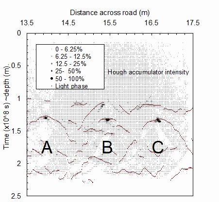
Fig. 2. Bright phase data pairs are shown by the dark circles. The Hough accumulator space in the variables Y and Z derived from these is superimposed as a grey scale. This has been normalized so that the maximum accumulator bin is black. Peaks in the accumulator space are seen close to each object A, B, and C.

In general, the more unknown variables to be found, the more correlated the solutions. Therefore, we begin with the simplest relevant case of a point object (R = 0) in soil whose radar velocity may at least be estimated at a value V=v. In this case, n = 2 and only doublet data pairs (y_i, t_i) and (y_j, t_j) need be chosen. The chosen points must be different, so that i <> j. Also note that when the points are different but very close, the solution will be ill-conditioned, and the solution will not be so accurate. The solutions for the unknown variables Y and Z

Y = [(y_i² - y_j²) - (t_i² - t_j²)v²/4)]/[2(y_i - y_j)]

Z = (vt_i/2)² - (y_i - Y)². (2)

In this case, the accumulator space is only 2-D and is easily plotted in real space [Y, Z]. Fig. 2 shows such an accumulator space for the bright phase data pairs of Fig. 1. The results are for 100 000 random choices of data pairs. The spatial resolution of the accumulator space DY = 0.02m in the direction of the scan, and DZ = 0.015m in depth. These values are comparable with the lateral step of 0.01m and the time sampling distance of 0.015 m. Many of the iterations are not recorded and do not result in any increment to the accumulator space. For example, the solution may be imaginary, or the range of the solutions may lie outside specified ranges of interest. It is seen from Fig. 2 that the accumulator space shows a number of significant dark areas indicating the positions of hyperbolic arc apexes, including each of the three principal hyperbolas denoted by A, B, and C in Fig. 1. There is also a background of ignorance at around the 10% level, covering most of the area near the apex points. This background arises from plausible solutions, arising from data pair choices where one point may lie on the hyperbola of interest but the other lies on a different hyperbola, on a noise signal or on a soil layer signal. The resulting background may center on the apex of interest, but extends at a relatively uniform level over a wide area.

IV. LABELING OF DATA-PAIRS USING A HOUGH ASSICIATIVE STORE

The accumulator space is conventionally an array with dimensionality equal to the number of unknown parameters. An integer array is conventionally chosen with each unknown variable being appropriately digitized with a step size DX_i for each variable X_i. An associative store is mathematically equivalent, but instead is a series of linear integer arrays, with one array describing the digitized value of each unknown parameter, and one accumulator array describing the number of hits for that set of variables X_i. Each Hough iteration, with a new random choice of data pairs and solutions X_i, first produces a fresh member j of the associative store, with an initial accumulator value of 1. However, after the first iteration, the solutions X_i are examined to see if any of the existing members of the store corresponds to the current solution. If this happens, then the existing accumulator value is incremented by 1. The associative method has many advantages in Hough solutions with highly peaked solutions. In this letter, a second associative store has been introduced with the objective of recording all contributing data pairs. It is composed of a new series of digital arrays whose index k is incremented for each recorded Hough iteration. For n unknown variables, these arrays record the indices j(i), i = 1, n of each of the n data pairs (y_j, t_j), contributing to each recorded iteration. A further index associates the recorded iteration number k with each bin j of the main associative store. The extra storage and computation causes no significant issues on a standard personal computer and the programs reported here run in only a few seconds.

The objective is to identify peaks in the Hough accumulator space and so to locate the contributing data pairs that define the hyperbolic arc arising from a given defect. The method used is to define for n unknown variables X_i a hyper-radius R= Sa_i (X_i-X_0i)², where the amplitudes a_i are chosen according to the spread of the variable to include the most appropriate cluster of large amplitude bins in the accumulator space. Bins lying within this radius are defined as belonging to the arc apex, provided that their amplitude is above a defined lower limit, say 20% of the peak amplitude. This figure is a compromise between including all the data pairs associated with a defect and rejecting false alarm pairs that only spuriously occur within the proscribed hyper-radius. In Fig. 3, the maximum included radius has been chosen as four bins along both Y and Z axes. These included bins are shown by closed squares, and the contributing data points from all bins defined as belonging to the apex are indicated by closed triangles. It is seen that the merged bins form a close cluster, and that the chosen contributing data pairs form a fair representation of the arc.

Fig. 3. Contributing data pairs for object C are shown by the closed dark triangles. The crosses are data pairs deleted by the threshold on contribution numbers. The results of a three-unknown parameter least-squares fit are shown. The full line is the best fit given by these parameters. At the top of the figure, the residuals are shown on a five-times expanded scale.

V. CONVENTIONAL LEAST-SQUARES FITTING TOFIND THE SOIL VELOCITY

Now that the data pairs contributing to object C have been delineated, conventional least-squares fitting to (1) becomes feasible. Since it is known that object C is an electric cable of only 0.04-m diameter, we may assume that it is a point scattering source (R = 0) and fit simultaneously to the three remaining parameters: object position Y, depth Z, and soil velocity V. This enables the radar velocity to be defined for this region of the soil as V = 1.142 x 108 ms^-1. Now that the first object hyperbola and its contributing points have been defined, a search may be made for further hyperbolas. However, since we have noted all the contributions to the accumulator space from the data pairs contributing to the first object, it is possible to scan through the whole of the accumulator space, searching for, and deleting, any contributions that have involved data pairs defined as belonging to this object. This clear-out process lowers the background of ignorance mentioned in Section III by removing those contributions arising from the first object hyperbola.

VI. FITTING A RADIUS TO THE CONCRETE PIPE B USING THE DARK PHASE DATA PAIRS

The concrete pipe is better defined from the dark phase data pairs, and the light circles in Fig. 4 show these as in the B-scan in Fig. 2. The grey scale shows the corresponding Hough accumulator space. This time, the highest bin in the accumulator space is for peak B and the dark squares show the merged high bins forming the cluster for apex B. A much bigger cluster of high bins is now present and a radius of eight bins proved necessary, twice the size used for the more compact peak C. The simulated shape of a 0.18-m radius pipe is shown in the right-hand top corner and confirms the larger size of the cluster expected. Once again, the number of contributions from each data point was thresholded. The closed triangles show the contributing points after thresholding and define the hyperbolic arc associated with this defect. The black crosses show the data pairs removed by thresholding. The thresholding process removed many data pairs whose affinity with the hyperbolic arc was dubious.

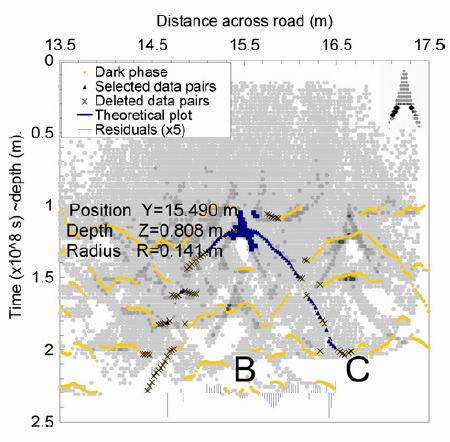
Fig. 4. Dark phase data pairs are shown by the light circles. The central object B gave the largest contributions to the Hough accumulator space, shown by the grey scale. The merged accumulator bins forming the apex are shown by the dark squares. The contributing data pairs for object B are shown by the dark triangles. The crosses are data pairs deleted by the threshold on contribution numbers. The results of a three-unknown parameter least-squares fit for the position Y , the depth Z, and the radius R at the velocity determined from peak C give the values shown in the figure. The full line is the best fit given by these parameters. At the base of the figure, the residuals are shown on a five-times expanded scale. At the top right in black, a simulation of a 0.18m pipe measured on a Y Z Hough transform shows the true form of the accumulator bin distribution.

This time, the velocity was assumed to be determined from object C, as described in Section VI. With V held at the value 1.142 x 10⁸ ms^-1 determined from this fit, a least-squares fit was made to the remaining three parameters: object position Y, depth Z, and pipe radius R. The full line shows the best fit to the contributing points, and the fitted parameters are shown. The fit of the theoretical line to the contributing points is good. It is noteworthy that the fitted radius of 0.14m is not far from the actual value of 0.18 m.

VII. CONCLUSION

A generalized Hough transform method for locating buried objects using radar was extended by recording in an associative store the position/time data pairs that form a contribution to any bin in the Hough accumulator space. By merging high bins in the accumulator space, and noting the data pairs that contribute to the peak, the data pairs lying on a hyperbolic arc attributable to a particular object may be defined. Having defined these data pairs, a conventional least-squares method may be used to determine unknown parameters of the object. Using real radar data from buried pipes, it was possible to identify two known pipes and to evaluate to 25% accuracy the diameter of a 0.36-m diameter buried concrete pipe at around 1-m depth.

ACKNOWLEDGEMENT

The authors would like to thank Prof. G. Borgioli, B. Morini, and Dr. S. Matucci for their useful comments and suggestions.

REFERENCES

[1] D. J. Daniels, "Surface penetrating radar for industrial and security applications," Microwave J., vol. 37, no. 12, pp. 68-82, Dec. 1994.
[2] J. H. Bungey and S. G. Millard, "Radar inspection of structures," in Proc. Int. Civ. Engnrs. Struct. Buildings., vol. 99. 1993, pp. 173-178.
[3] M. M. Golovko and G. P. Pochanin, "Automatic measurement of ground permittivity and automatic detection of object location with GPR images containing a response from a local object," in Ultrawideband Radar: Applications and Design. Gainesville, FL, USA: J. D. Taylor Associates/CRC Press, May 2012.
[4] T. Imai, T. Sakayama, and T. Kanemori, "Use of ground-probing radar and resistivity surveys for archaeological investigation,2 Geophysics, vol. 52, no. 2, pp. 137-150, Feb. 1987.
[5] D. J. Daniels, "A review of GPR for landmine detection" Int. J. Sens. Imaging, vol. 7, no. 3, pp. 90-123, Sep. 2006.
[6] E. M. Johansson and J. E. Mast, "Three-dimensional ground-penetrating radar imaging using synthetic aperture time-domain focusing," in Proc. SPIE Advance. Microwave Millimeter Wave Detectors, vol. 2275. 1994, p. 205.
[7] E. Pasolli, F. Melgani, and M. Donelli, "Automatic analysis of GPR images: A pattern-recognition approach," IEEE Trans. Geosci. Remote Sens., vol. 47, no. 7, pp. 2206-2217, Jul. 2009.
[8] C. Windsor, L. Capineri, and P. Falorni, "The classification of buried pipes from radar scans," INSIGHT, J. Brit. Inst. Non Destruct. Testing, vol. 45, no. 12, pp. 817-821, Dec. 2003.
[9] R. O. Duda and P. E. Hart, "Using the Hough transforms to detect lines and curves in pictures," Commun. ACM, vol. 15, no. 1, pp. 11-15 Jan. 1972.
[10] T. C. K. Molyneaux , S. G. Millard, J. H. Bungey, and I. Q. Thou, "Radar assessment of structural concrete using neural network," NDT Int., vol. 28, no. 5, pp. 281-288, 1995.
[11] K. Deguchi, T. Okada, and I. Morishita, "Analysis of underground radar image using generalized Hough transformation technique," Trans. Soc. Instrum. Control Eng., vol. 25, no. 7, pp. 72-75, 1989.
[12] F. C. Morabito and M. Campolo, "A novel neural network approach in non-destructive testing," in Proc. 3rd Int. Conf. Comput. Electromag., IEE Conf. Publ. no. 420. Apr. 1996, pp. 364-369.
[13] M. R. Shaw, T. C. K. Molyneaux, S. G. Millard, M. J. Taylor, and J. H. Bungey, "Assessing bar size of steel reinforcement in concrete using ground penetrating radar and neural networks," Insight Non- Destruct. Testing Condition Monitoring, vol. 45 no. 12, pp. 813-816, 2003.
[14] R. Hunik, "Detection and sizing of cables and leads with sub-surface radar," in Proc. 12th World Conf. Non-Destructive Testing, 1989, pp. 1261-1266.
[15] C. G. Windsor and L. Capineri, "Automated object positioning from ground penetrating radar images, INSIGHT," J. Brit. Inst. Non Destruct. Testing, vol. 40, no. 7, pp. 482-488, 1998.
[16] L. Borgioli, P. Capineri, S. Falorni, Matucci, C. G. Windsor, "The detection of buried pipes from time-of-flight radar data," IEEE Trans. Geosci. Remote Sens., vol. 46, no. 8, pp. 2254-2266, Aug. 2008.
[17] G. Manacorda [Online]. Available: http://www.giga-radar.info/docs/ Manacorda.htm