Euratom-UKAEA Fusion Association, Culham Science Centre, Abingdon, OX14 3DB, UK*

Euratom-Max-Planck-Institut fur Plasmaphysik, Garching, D-85748, Germany

*Pamela, J. et al., Annex 1, Overview of recent JET results, Fusion Energy 2002 (Proc. Int. Conf., Lyon, 2002), Nuclear Fusion, 43, 1540, 2003.

Accepted for publication 15/3/2005

Abstract

First results are reported on the prediction of disruptions in one tokamak, based on neural networks trained on another tokamak. The studies use data from the JET and ASDEX Upgrade devices, with a neural network trained on just 7 normalised plasma parameters. In this way, a simple single layer perceptron network trained solely on JET correctly anticipated 67% of disruptions on ASDEX Upgrade in advance of 0.01 seconds before the disruption. The converse test led to a 69% success rate in advance of 0.04 seconds before the disruption in JET. Only one overall time scaling parameter is allowed between the devices, which can be introduced from theoretical arguments. Disruption prediction performance based on such networks trained and tested on the same device shows even higher success rates (JET: 86%; ASDEX Upgrade 90%), despite the small number of inputs used and simplicity of the network. It is found that while performance for networks trained and tested on the same device can be improved with more complex networks and many adjustable weights, for cross machine testing the best approach is a simple single layer perceptron. This offers the basis of a potentially useful technique for large future devices such as ITER, which with further development, might help to reduce disruption frequency and minimise the need for a large disruption campaign to train disruption avoidance systems.

1. Introduction

Disruptions [1,2] are a key design issue for tokamaks, limiting their operational domain. They naturally arise in tokamaks, particularly when new regimes or techniques are explored, performance limits are pushed, or particular systems fail. On present day tokamaks disruptions are generally tolerable. However on future power-plant scale devices, such as ITER, only a limited number of disruptions will be tolerable - concerns range from reduced device lifetime to possible structural damage. In a disruption the plasma thermal energy is lost rapidly with the result that the plasma position and shape changes, causing the plasma to interact with the containment vessel walls, and dump its current over a very short period. The resulting eddy and halo currents in the device structure interact with the high magnetic field to create large mechanical forces that may require the imposition of operational and design constraints. Serious concerns are also posed by the accompanying heat load on plasma facing components and the potential for creating a narrowly focused 'runaway' electron beam.

Thus disruption avoidance, or mitigation, is highly desirable, and it is prudent to consider how our knowledge of the circumstances of disruptions in a given tokamak could be used to predict disruptions in another tokamak. If successful, this approach would allow the deployment of disruption protection systems in future tokamaks, such as ITER, without the need to have a large number of 'training' disruptions in that device. It would also enable that device to operate in a more cautious manner, until the safety of particular scenarios was established.

The starting point of such a study is the search for plasma diagnostic parameters that are indicative of disruptive behaviour. A great deal of progress has now been made in this field using the ASDEX Upgrade (AUG)[3], DIII-D[4], COMPASS-D, JET[5] and JT-60U[6], TEXT[7,8] and ADITYA[9] tokamaks. These studies indicate that for around 80% to 90% of disruptive shots the time of disruption can be predicted early enough to take corrective action. They also show a considerable measure of agreement over the best choice of parameters.

These previous studies have all used neural network classifiers [10] for the prediction of disruptions. Neural classifiers use a database of historical data where each example is a set of plasma parameters from a given time in a given shot. During network training each training example item is associated with a 'target' indicating the time to disruption, or some function of it. The parameters of the network are adjusted during the training process until, for each set of training example inputs, the network outputs most closely match their targets. The trained network can be used in subsequent testing sessions to predict the time to disruption for any new set of example parameters. Essentially the network searches the multi-dimensional space of the chosen plasma parameters for previous examples having parameters close to the current values of the parameters, and assumes that the subsequent evolution of the plasma will be similar. It should be noted however that neural network application developed here is unique in that the training and testing data are from 2 completely distinct sources (i.e. two different tokamaks). There is therefore a degree of extrapolation required by the network, as the data ranges of the two devices are not entirely overlapping. In this paper, we start with a discussion of the basis of our approach, key parameters used, and description of the databases used. We then explain the neural network learning and testing procedure. To present results, we first explore performance based on training and testing within a single device, considering first ASDEX Upgrade, then JET. This then sets the framework for an evaluation of cross-machine prediction, which is performed in each direction. We then present our conclusions.

2. Basis of the approach

For comparison between tokamaks of differing size and structure to be valid, the plasma parameters must be made dimensionless. Some parameters, for example the edge safety factor, q95, are intrinsically dimensionless. Other possible parameters such as the radiated plasma power can be made formally dimensionless by dividing by say, the plasma input power, to define a radiated power fraction parameter. In this work we do not allow further adjustment factors in scaling dimensionless parameters between devices.

The normalised plasma parameters used here are based on quantities that are known to play a role in tokamak plasma disruptivity. They are largely based on those used in the ASDEX Upgrade disruption prediction [11,12], with three changes. (i) The MARFE (Multi-faceted Asymmetric Radiation From the Edge) indicator used as one of the ASDEX Upgrade parameters had no exactly equivalent on JET, so this variable was not used. (ii) The time differential variables were not used. (iii) It was found that the confinement time in the present application was more predictive when normalised by a simple average confinement time over the relevant tokamak database than by the L-mode confinement time scaling law of Franzen et al. [13] used in the ASDEX Upgrade work. This is partly because such scaling laws depend on parameters which are sometimes varying in the approach to a disruption, normalising actual time to confinement law scaling time can lead to considerable fluctuation in the normalised time input parameter. Results will be given for the network performance trained using a smaller dataset containing only a logarithmically spaced selection of times before any disruption and using a new target with a dimensionless time variable. Testing is performed on different datasets containing a much larger number of time points at a uniform spacing.

2.1 Network input parameters:

The normalised plasma variables to be used in disruption studies are defined as follows:

1. The edge safety factor: P₁ = q₉₅. This is the value of the safety factor at the 95% flux surface. A low value (<~3) is indicative of disruptive behaviour.

2. Internal inductance: P₂ =l_i. This is the ratio of the average value of the magnetic field over the average value of the field at the plasma edge. It therefore is also dimensionless. A high value of the internal inductance is known to increase the likelihood of disruption [2].

3. The normalised toroidal beta: P₃ = b _N = bT /(I_p[MA] /a[m] B_T[T] ) with b_T = 2m₀/B_T and the normalisation depending on the plasma current (I_p) the minor radius p(a) and the toroidal field (B_T ) arising from the predicted Sykes-Troyon b-limit [1]. Sawtoothing ELMy H-mode plasmas tend to become unstable if the parameter P₃ rises above about 3.5.

4. The Greenwald density limit P₄ = n_N = n_e/ I_p/ (pa²k). Here n_e is the measured line average density, and I_p/( pa²k) is a generalised Greenwald density including the elongation k. A high value of P₄ (>~k) increases the probability of a disruption via radiative collapse.

5. The radiated power fraction: P₅ = P_frac = P_Rad / P_Inp. Here P_Rad is the radiated power from the plasma determined from bolometer measurements. P_Inp is the input power from external and Ohmic heating. A high radiated power fraction (>~100%) is characteristic of disruptive activity.

6. The normalised energy confinement time: P₆ = t_N = t_con/<t_con>. The confinement time is calculated from the stored energy, divided by the total energy, less the time derivative of the energy. The confinement time is normalised according to the average value over the dataset, so this is not an H factor. A low normalised confinement time is suggestive of a disruptive plasma.

7. The normalised locked mode indicator: P₇ = L_n. The signal is normalised to a maximum value of unity so that it switches rapidly from zero (no locked mode) to unity (locked mode present).

2.2 The databases used for ASDEX Upgrade and JET

The ASDEX Upgrade disruption database used consists of ELMy H-mode shots selected from 1,400 pulses with lower single-null plasmas and a flat-top current. Shots were omitted if they contained incomplete or unreliable measurements. Disruptions caused by killer pellets or vertical displacement instabilities were also excluded (as these represent machine specific causes that will vary according to specification between devices). The training set included values of chosen variables measured every 0.0025 seconds. Generally times up to 0.8 seconds before any disruption were included. A complementary set of non-disruptive shots were selected to provide a broader definition of the non-disruptive parameter space. For our study only those disruptive shots where parameters were recorded for at least 0.067 seconds before the disruption were included. For training data not all times were used. Since the disruption-significant variables change rather rapidly just before the disruption, but less rapidly at much earlier times, an equal spacing of time points gives an inefficient picture of the approach to the disruption. Variables at adjacent time points well before a disruption tend to be highly correlated with each other, potentially leading to excessive training in the time region well before the disruption while sparsely representing the important data close to the disruption. A logarithmic time variation was therefore chosen with the earliest time 0.005 seconds before the disruption and earlier times at intervals of 2^1/2 times the previous time. This ratio was a compromise between adequate representation of the time variation up of the variable up to the disruption and the avoidance of large numbers of correlated points. The idea is to create a dataset where the features at each example point are only poorly correlated with those of its immediate neighbours. Instead of around 185 time points for each disruptive shot, there are now just 16 spanning a time range up to 0.64 sec. before the disruption. We suggest that this relatively small number of example points, moving smoothly from a long time before a disruption to fine time resolution just before it, nicely captures the essence of the disruptive behaviour. The time points in non-disruptive training points were randomly chosen so as to give a similar number of time points. The result was a database of 1101 sets of variables (time points) from 59 disruptive shots and 30 non-disruptive shots in ASDEX Upgrade.

A quite separate database was created for testing purposes, since it was realised that the large time intervals in the training data well before a disruption might permit short lived excursions towards disruptive behaviour leading to false alarms being missed. For this reason all time points were included in the test database provided that they originated from a plasma current flat top region of the shot. This testing database contained some 17,967 time points.

The JET database was generated from a list of ELMy H-mode disruptive shots and excludes those caused by loss of vertical control. From these, only shots with disruptions in the plasma current flat-top region were chosen. Non-disruptive shots were chosen to correspond closely with the plasma conditions of some of the disruptive shots. Once again the parameters at logarithmically spaced time intervals were chosen for training, with the first time 0.01 seconds before the disruption and the last 3.2 seconds before the disruption. This gave again around 15 training points spanning the time range before the disruption. There were 1290 sets of variables from 68 disruptive shots and 18 non-disruptive shots in the final training database. Again a separate test database of 41,100 time points was constructed containing all the time points within the flat-top region of the selected shots.

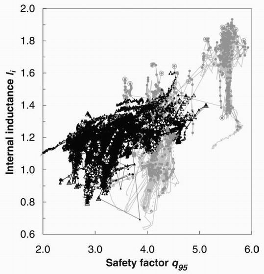
Figure 1. The scatter plot of the internal inductance against the safety factor for ASDEX Upgrade (feint circles) and JET (dark triangles) disruptive and non-disruptive shots. The larger symbols are just prior to the disruption. The dashed lines are for non-disruptive shots.

An example of the type of scatter plot used initially to define potential variables for disruption prediction is shown in figure 1. This is a plot of the internal inductance l_i against the safety factor q95 which Wesson [2] and Milani [5] have emphasised as a defining diagram to separate regions of stability and instability.

3 The neural network learning and testing procedure

The neural network which has run on-line on ASDEX Upgrade [12] used the time to disruption (in seconds) as its target and was able to predict around 85% of the disruptions (based on a different success criteria to that used in this paper). A first objective of the present work was to confirm these results using a revised target involving a time to disruption normalised by the average confinement time for a given device. The revised target used has the form:

T = exp{ -F(t_dis - t) / <t_con>} (1)

Here t is the time, t_dis is the disruption time and F is an arbitrary factor, typically about 8. <t_con> is the average confinement time over the dataset as defined earlier in the definition of the normalised energy confinement time. This target has the advantages that it smoothly approaches 1 as the disruption is approached and smoothly decays to zero at times far from any disruption. It can readily be given the value 0 for any times within non-disruptive shots. The factor F can be adjusted, as described later in Section 6, so that optimum predictive performance is achieved with the largest target variation occurring at those times when the network is most predictive.

In any "learning by example" procedure great care has to be taken to ensure the optimal position between the twin evils of using too many adjustable parameters so that unimportant details in the training data are "over-learnt", and using too few parameters so that even general trends in the training data fail to be followed. In the multi-layer perceptron networks discussed here the key variable is the number of weights in the network. For a two-layer network of n₀ input variables, n₁ hidden layer neurons and a single output neuron n₂=1, the number of adjustable weights is

n_wts = n₀ .( n₁ +1) + n₁ +1 (2)

The number of weights can therefore be adjusted by changing the number of hidden neurons n₁ , and also reduced by cutting out input variables n₀. A further step is to eliminate the hidden neuron layer altogether to make the single-layer perceptron, where the single output neuron 0₁, receives signals o_0ik input from each of the inputs i, of example k, multiplied by the weights w_i, less a threshold w_i0

0_k = G{ [S_i o_0ik.w_i ] - w_i0 } where G{x} =1/[1+ exp( -x/kT_B )]. (3)

Here G(x) is the non-linear function of the argument x, changing from zero for large negativex to 1 for large positive x. T_B is a pseudo-temperature defining the degree of smoothness of the transition. In the present code the single-layer perceptron, n₁=0, is treated as a continuation of the finite hidden unit number series. During the learning process all the adjustable weights are varied iteratively to reduce the "output" residual, R₀, between the actual outputs o_k for each training example k and the known targets T_k.

R₀ = S_k (o_k - T_k )² (4)

The summation here is taken over all examples in the data, in contrast to that in the "time residual" used later in equation (5) where the summation is only over times of interest in predicting the disruption. The learning rate must be slow enough to ensure a smooth reduction of the residual R₀ in Eqn (4) and the number of iterations large enough to ensure reasonable convergence. When we are considering examples from a single tokamak, the available examples can be divided into training and testing example datasets. However a better way is to perform "leave-one-shot-out" testing where the network is trained from scratch with just one shot left out of the training data, and subsequently tested on the data from this shot alone [17]. The process is then repeated leaving out each shot in turn, so that a statistic measuring performance against all shots can be compiled. This method has been used exclusively in this work for the single tokamak studies. For the inter-tokamak studies that are the main subject of this work, the complication does not arise. One tokamak supplies training data and another the test data.

A neural network code incorporating the standard Rumelhart and McClelland back propagation algorithm [15], was written in 1990 as part of the European ESPRIT II project 'Applications of Neural Networks for Industry in Europe' [16]. This has been developed to allow leave-one-shot-out testing and to allow a smooth transition to zero hidden units.

The convergence of the network was tested by performing a scan of test performance against the number of iterations. Our code was written so that any of the neural network performance parameters could be automatically scanned and the full test performance noted. These tests were performed on the ASDEX Upgrade alone run 1 of Table 1. The test failure rate improved up to 300,000 iterations but showed little improvement with more iterations. The best results were for 600,000 iterations and this value was used in all the results shown. For cross-tokamak training and testing, this conclusion would not be valid. The cross-tokamak test performance with several hidden units is improved by using say 60,000 instead of 600,000 iterations. However its performance still falls below the zero hidden unit network. Tests were also made with the learning rate - i.e. the rate at which the neural network weights are changed after each iteration in the back propagation formalism of Rumelhart and McClelland [15]. A low learning rate is best but most time consuming. A high value can give problems of instability shown by a residual which fluctuates rather than reducing steadily. The learning rate was initially set to 1.0 with 300,000 iterations. An appreciable improvement was obtained by reducing this to 0.5 and doubling the number of iterations to 600,000. However a further factor of two change with more iterations and still lower learning rate produced little further improvement. A scan was made of the factor F in equation 1, which multiplies the time-to-disruption before evaluation of the exponential in the target. It was found that the residual decreased rapidly as the factor increased from 1 to around 8 but then showed little further change. No momentum term in the back propagation formalism of Rumelhart and McClelland [15] was used.

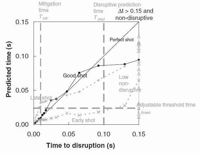
Figure 2. The time-to-disruption plot used to classify disruptions. A successfully predicted disruption (full circles) has a trajectory passing below T_thres between times T_mit and T_pred. "Early" predictions, or false alarms, (crosses) fall below T_thres before T_pred. "Late", or missed, predictions (plus signs) fall below T_thres only after T_mit. Points in non-disruptive shots (triangles) are defined as failures if their trajectory falls below T_thres at any time. A perfect prediction would follow the line of unit gradient.

Network performance testing can be refined beyond the residual of equation 4 to include the factors that make the prediction of disruption in a particular shot practically useful or not. These are illustrated in figure 2, which shows the predicted time to disruption, evaluated by inverting equation 1, against the actual time to disruption for several shots. A 'perfect' prediction would give a trajectory following the unit gradient line shown. An adjustable threshold time T_thres shown by the horizontal dashed line is used to define the onset of a disruption. The vertical dashed line to the right of the figure defines the prediction time T_pred, before which shots are considered to be non-disruptive. The vertical dashed line to the left of the figure represents the mitigation time T_mit after which it is too late to perform any actions to mitigate the effects of the disruption. This time has been chosen relatively arbitrarily and is not based on any particular mitigation method. We shall define 4 types of shot:

a) An 'early' failure shot has a predicted time to disruption falling below T_thres for actual times earlier than T_pred.

b) A 'late' failure shot has a predicted time to disruption failing to fall below T_thres for any actual times before T_mit. In our code a shot which is both 'early' and 'late' is defined as a 'late' shot.

c) An "non-disruptive" failure shot occurs if the predicted time to disruption falls below T_thres at any time.

d) A 'good' shot has a predicted time to disruption falling below T_thres for actual times somewhere between T_mitTmit and T_pred or for a non-disruptive shot, the predicted time must remain above T_thres for all times.

Performance is defined as the (number of 'good' shots)/(total number of shots). The failure rate is defined as (1 - performance) and can be subdivided into 'early', 'late' and 'non-disruptive' failure rates.

The choice of T_mit and T_pred depends on the tokamak, and both are critical to the performance results. In ASDEX Upgrade there is experience in disruption mitigation by impurity gas injection[12]. Values that are consistent with the present hardware are a mitigation time T_mit=0.010 seconds and a prediction time T_pred=0.100 seconds. For JET the figures will be corresponding longer. In the work of Cannas et al. [14] on JET, T_mit was scanned between 0.04 and 0.20 seconds and the lowest number of missed alarms found was at 0.04 seconds. T_pred was chosen as 0.440 seconds. Here we have used the (minor radius)² scaling to give a consistent factor 4 time ratio between JET and ASDEX Upgrade. This gives the values T_mit=0.040 seconds and T_pred=0.400 seconds, consistent with the work of Cannas et al.. This mitigation time is of the order that is sufficient to allow an adequate mitigation strategy. Note that the figures have a time axis extending to 20% above T_pred to give clarity to the time region close to the disruption. The actual range of the considered time points extends to many times this value. Time points greater than this limit are superimposed on the right-hand axis and are included in performance statistics. Later in figure 9 we show some example inter-tokamak predictions using such an expanded time scale.

Table 1. A numerical resume of disruption prediction performance results for single tokamaks

Run	Tokamak	Training	Hidden	Output	Time	Threshold	Best %	Early %	Late (%)	Non-d (%)
-	-	-	units	residual	residual	(secs)	failure	failure	failure	failure
1	AUG	leave-one-shot-out	0	0.085	0.164	0.025	8.89	4.44	3.33	1.12
2	AUG	hidden unit scan	6	0.067	0.015	0.019	7.78	3.33	3.33	1.12
3	AUG	Saliency:1 -Pfr	0	0.141	1.010	0.027	32.58	17.98	14.61	0.00
-		Saliency:2 -Tau	0	0.121	1.277	0.029	25.84	17.98	7.87	0.00
-		Saliency:3 -li	0	0.117	0.730	0.027	15.73	10.11	4.49	0.00
4	JET	leave-one-shot-out	0	0.043	0.000	0.096	13.64	3.41	10.23	0.00
5	JET	hidden unit scan	8	0.080	0.327	0.058	12.50	2.27	10.23	0.00
6	JET	Saliency:1 -Tau	0	0.119	0.568	0.088	50.00	38.64	11.64	0.00
-		Saliency:2 -Loc	0	0.069	0.349	0.124	18.18	7.95	7.95	0.00
-		Saliency:3 -Pfr	0	0.057	0.387	0.076	18.18	7.95	10.23	0.00

4. Results for training and the leave-one-shot-out testing with ASDEX Upgrade

Table 1 shows the results of several optimisations performed on the ASDEX Upgrade data alone and JET data alone, giving time residuals, success rates and optimum threshold times. The "reference" calculation includes all 7 parameters and is performed with the no-hidden layer simple perceptron, and with leave-one-shot-out testing. Three independent measures of performance are used in Table 1. These are the output residual of equation 4, the total percentage of shots not correctly classified, and a "time" residual, Rt, equal to

R_t = S_k | (t_nn - t_actual)/t_actual| (5)

Where t_nn and t_actual are the neural network predicted and actual times to disruption, and the summation only runs over times between T_mit and T_pred for disruptive shots, and over all times for non-disruptive shots. Figure 3 shows, for the ASDEX Upgrade shots, the predicted time to disruption plotted against the actual time to disruption for times up to 0.12 sec.

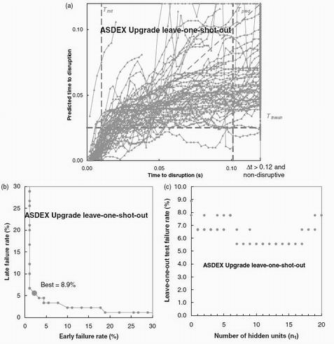
Figure 3 (a). The actual time to disruption from ASDEX Upgrade shots plotted against the predicted time for leave-one-shot-out testing. Included times in disruptive shots above the axis time limit, and all non-disruptive data are plotted down the right hand axis. (b)A performance plot of the number of "late" disruption prediction errors against the number of "early plus non-disruptive" errors as T_thresh is varied. The heavy point indicates the best value of the threshold time, and the lowest failure rate is indicated by 'Best'. (c). A plot of the time-residual between actual and predicted times to disruption as a function of the number of hidden units.

The lines in figure 3a shows the ASDEX Upgrade time-to-disruption plots in the style of figure 2 for leave-one-shot out-training. Perfect performance of the neural network would result in all trajectories lying on the y=x line. The resulting 8.9% overall failure rate of this network, which is given by a simple sum of 'early', 'late' and 'non-disruptive' failures, arises from 4 'late', 3 'early' and one non-disruptive shots. One 'late' shot is seen falling steeply on the extreme upper-left of the figure. The two 'early' shots are nearly flat at the bottom of the figure. Despite this good performance it is seen that the time-to-disruption traces have a systematic trend away from the expected unit gradient, most notably for times further away than about 0.04 seconds or so from the disruption. The predicted time to disruption tends to flatten off at about 0.06 seconds. We believe this to be caused by the decreasing disruption predictive behaviour of the input parameters. At a sufficiently long time before a disruption there is little distinction between the input parameters from disruptive and non-disruptive shot. For a single tokamak, predictive power is generally increased by a more complex network with more hidden units. A 6-hidden unit multi-layer perceptron, detailed as Run 2 in Table 1, gives a slightly reduced output residual and error rate. We detail the single-layer perceptron results here for comparison with the inter-tokamak results presented later. The horizontal line in figure 3a shows the threshold time giving the best overall performance. This value has been determined as in figure 3b by changing the threshold over a wide range and examining the number of 'early' and 'late plus non-disruptive' errors. There is generally a minimum where the threshold is neither too low to prevent indications of 'early' disruptions or false alarms, nor so high to prevent the indication of a true disruption. Figure 3c shows how the performance changes as the number of hidden units is increased. With more than 6 hidden units, the performance is improved. This result is consistent with other studies where optimal performance on a given tokamak has been achieved using networks with several hidden units. [3]

Table 2. The saliency table showing the prediction failure rate as each of the input parameters is omitted in turn.

-	Train tokamak	ASDEX-U	JET	ASDEX-U	JET
-	Test tokamak	ASDEX-U	JET	JET	ASDEX-U
All	Failure rate (%)	8.9	13.6	29.6	26.7
1	Q95	11.2	13.6	29.6	27.8
2	li	15.7	15.9	31.8	34.8
3	Normalised beta	10.1	15.9	30.7	27.8
4	Normalised density	13.5	15.9	30.7	50.0
5	Power fraction	32.6	18.8	34.1	24.4
6	Confinement time	25.8	50.0	78.4	30.0
7	Locked mode	14.6	18.8	34.1	66.7

Table 2 shows the saliency analysis when each of the input parameters are omitted in turn, and the usefulness of each one evaluated from the deterioration in the performance. This shows that all parameters are useful when tested on the ASDEX Upgrade data. It should be noted here that the saliency test is against the failure criteria (Fig 2) whereas the network performance is optimised against the residuals. Results for networks corresponding to the three most salient parameters of Table 2 are shown in 'Run 3' of Table 1.

It is interesting that almost identical results are obtained when all the available ASDEX Upgrade data is used for training. The similarity between this '100% learning' case and the leave-one-shot-out analysis, shows that there is little tendency for these small networks to exhibit the 'over-learning' behaviour typical of larger networks. They have only 8 adjustable parameters (7 feature parameter weights and a threshold weight), compared with say 78 for a 7-input, 10-hidden unit multi-layer perceptron. The larger number of variable weights in the multi-layer perceptron allows the training to pick out unimportant details in the training dataset to minimise the residual between the target and the network output. These details may well not occur in testing so that the extra precision of the training cannot be used and the network is said to be 'overtrained'

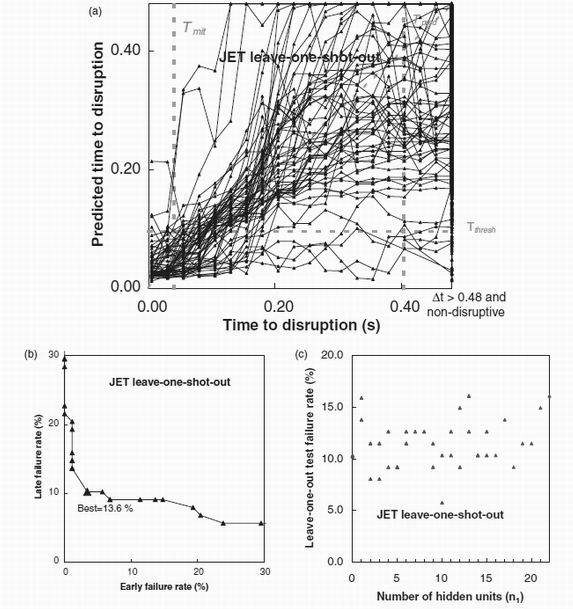
Figure 4. A corresponding plot to figure 3 for the JET database.

5. Results for training and the leave-one-out testing with JET

Corresponding results to AUG are shown from JET in Figure 4. For the present, it will be assumed that the JET time normalisation (in Eq. 1 and parameter P₆) is a factor 4 greater than for ASDEX Upgrade. This multiplier is consistent with a (minor radius)² scaling. Theoretically, this might originate from arguments relating to the resistive nature of the disruption process. For example a resistive evolution of the current profile towards disruption. [2]) . The resistive time constant of the plasma would be expected to scale with (minor radius)². Its role will be explored in more detail later in this paper. Table 1 also shows the JET data results. They show slightly worse performance than the ASDEX Upgrade data (13.6 % failure rate versus 8.9 %). The reason for this could well be the greater variety of shot types included in the JET database. These results can be compared with those of Cannas et al. [14] on JET which showed around 9% errors for similar times for the mitigation time T_mit = 0.04 seconds and the prediction time T_pred = 0.44 seconds. The predicted times to disruptions of figure 4a follow the correct trend quite well below 0.2 seconds. The hidden unit dependence is similar to that observed for ASDEX Upgrade, again showing an improvement in performance up to about 10 hidden units. Table 2 shows that most variables are of some use, and none decrease performance. The normalised confinement time is the most important parameter. Table 1 (runs 1 and 5) shows that the optimum threshold for JET is a factor 3 over that of AUG, not too far from the overall factor 4 between time normalisation between devices assumed above. The relatively high maximum values of the input parameters safety factor q95, normalised toroidal beta and normalised density suggest that the database includes shots not far from several types of disruptive behaviour.

Table 3. The ranges of the 7 parameters in the two tokamaks

-	Parameter	AUGmin	AUGmax	JETmin	JETmax
1	Q95	3.111	5.930	1.932	5.123
2	li	0.745	1.932	0.692	1.498
3	Normalised beta	0.123	2.975	0.060	4.282
4	Normalised density	0.016	5.081	0.197	3.266
5	Power fraction	0.086	4.000	0.009	3.066
6	Confinement time	0.052	8.108	0.023	4.144
7	Locked mode	0.000	1.000	0.003	1.000

6. Extending techniques to cross-machine prediction, and network optimisation

The ultimate purpose of this study is to predict the disruption performance of a new tokamak having no database of disruptions. Testing with data from a new tokamak should therefore not depend on any threshold, or other performance parameter depending in any way on the test data. In the present application this means there are no problems with the division between training and testing data. All the ASDEX Upgrade data can be used for training and all the JET data can be used for testing (or vice-versa). However some new complexities are introduced. In neural network training it is usual to normalise the input parameters into the range 0 to 1 and this has been done for each tokamak in the previous two sections. The actual non-normalised ranges of the 7 input parameters are shown on the left hand side in Table 3. As discussed later, they vary appreciably between the two tokamaks although the extremes of the range are often caused by one or two unrepresentative shots. It follows that the range appropriate for training the ASDEX Upgrade data is inappropriate for use in testing the JET data. It was found that a good strategy was to use the range appropriate to the test tokamak, whatever the training tokamak range. This means that for application to new devices (e.g. ITER), although no actual disruption data is required, the likely operating range of that device must be anticipated.

Related to this problem is the choice of time scaling factor between the devices, used in Eq. (1) and the definition of normalisation of the 6th parameter, the normalised confinement time, P₆. A good starting point, mentioned in section 5, is to use (minor radius)² scaling giving a factor close to 4 for JET compared to ASDEX Upgrade. It was less satisfactory to use actual averages of confinement time over the two databases, as there was no certainty that the shots in the two databases from each tokamak correspond to sufficiently similar scenarios, and it also requires anticipation of the average confinement time on the test device. A third choice is to treat the JET/AUG mean confinement time ratio as an adjustable parameter in the inter-tokamak predictions we compare this approach with the above minor radius assumption, below. In section 3, the origins for the choices of mitigation and prediction times (T_mit and T_pred) were given, based on previous work and on the ASDEX Upgrade practical experience. For the purposes of inter-device comparisons in this paper we have always maintained the ratio between devices of each of these times to be fixed, equal to the overall time ratio discussed above. For a future device, neither of these parameters are required for the operation of a predictive network - only for evaluating its success (whether disruption predictions are too early or too late). However, for testing on a future device, T_mit will depend on the physics processes associated with the chosen termination system (eg a massive gas puff), while T_pred could be further optimised to give best performance on the training device, before being scaled to the test device. We have not explored such variation in this work, and this remains an issue for the future.

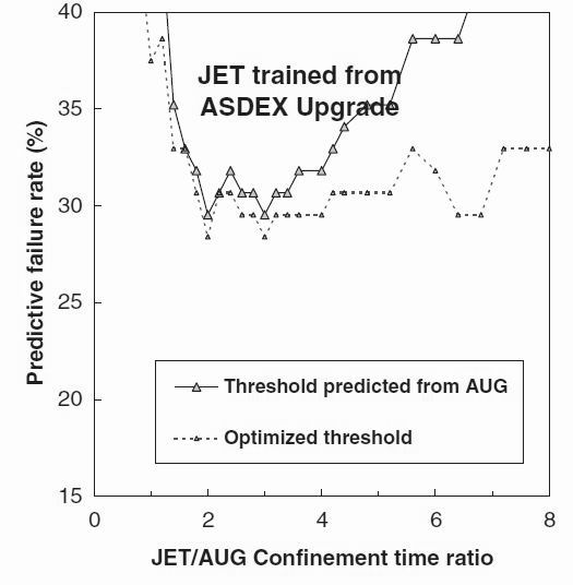
Figure 5 : The disruption prediction failure rate for JET data tested using a network trained on the ASDEX Upgrade data, as a function of the time ratio between JET and ASDEX Upgrade. The full curve shows the predicted JET performance at the best ASDEX Upgrade threshold (T_thres) as the time ratio between devices is varied. The light dashed curve shows the JET performance if the JET threshold is independently optimised. The plot shows the expected minimum around 4, - the value expected from the ratio of the square of the minor radii of the tokamaks.

The full line in figure 5 shows the disruption prediction performance for the JET data trained on ASDEX Upgrade data, with a threshold equal to that giving the best performance on the ASDEX Upgrade training data scaled by the particular confinement time ratio. It is seen that the expected minimum around a value from 2 to 4 is achieved with a failure rate of 29.4 % . The dashed line shows the improved performance for JET data trained on ASDEX Upgrade that could be obtained if the JET time threshold for disruption prediction is optimised independently for each possible value of cross-device time scaling factor. The failure rate is decreased to 28.4 % at a confinement time ratio of 3.0.

Table 4. Results for disruption prediction performance between tokamaks

Run	Training	Run	Hidden	Train (%)	Testing	Output	Time	Threshold	Best %	Early %	Late (%)	Non-d (%)
-	Tokamak	-	units	Failure	tokamak	residual	residual	(secs)	failure	failure	failure	failure
7	AUG	JET best prediction	0	3.37	JET	0.047	0.046	0.128	30.68	13.64	15.91	1.12
8	AUG	JET time ratio=3.0	0	7.78	JET	0.003	0.158	0.116	28.41	12.50	14.77	1.12
9	AUG	hidden unit scan	10	5.56	JET	0.044	0.916	0.104	46.59	15.91	29.55	0.00
10	"	Saliency:1 -TauN	0	13.33	"	0.141	0.158	0.072	72.73	37.50	32.95	0.00
-	"	Saliency:2 -DenN	0	8.89	"	0.003	0.158	0.100	35.23	19.32	14.47	0.00
-	"	Saliency:3 -locked	0	8.89	AUG	0.006	0.158	0.124	35.23	17.05	17.05	0.00
11	JET	AUG best prediction	0	32.95	AUG	0.055	0.038	0.036	26.67	16.67	5.56	0.00
12	JET	AUG time ratio=2.4	0	28.41	AUG	0.054	0.045	0.042	21.11	12.22	4.44	0.00
13	JET	hidden unit scan	10	30.68	AUG	0.044	0.180	0.056	45.56	40.00	1.11	0.00
14	"	Saliency:1 -Locked	0	10.45	AUG	0.049	0.646	0.051	65.56	64.44	0.00	0.00
-	"	Saliency:2 -DenN	0	40.91	"	0.032	0.052	0.054	51.11	46.67	0.00	0.00
-	"	Saliency:3 -li	0	36.36	"	0.054	0.054	0.061	47.78	25.56	2.22	0.00

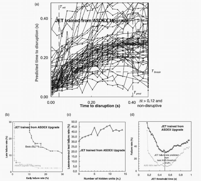
Figure 6. The plots corresponding to figures 3 and 4 for JET data tested using a network trained on the ASDEX Upgrade data. All variables have been included in this test. A simple perceptron with 100% learning has been used with a JET/AUG confinement time ratio of 4. In (b) the large triangle indicates the disruption threshold time giving the best performance. The feint points and line show the training data performance. In (c) the deterioration of performance with increasing hidden unit number is shown. In (d) the performance figures are shown plotted against the threshold. The optimal threshold plot shown in previous figures has limited validity, as for a future tokamak there may exist no database over which to vary the threshold.

7. Results, training on ASDEX Upgrade and testing on JET

Details of the inter-tokamak predictions are given in table 4, with summaries of the prediction of JET disruptions by an ASDEX Upgrade trained network given in figure 6. In this figure the predicted threshold scaled from the ASDEX Upgrade training, corresponding to the full line in figure 5(a) has been used. In figure 6(a) it is seen that, below around 0.2 seconds, the calculated times to disruption move with more-or-less the correct gradient. However they are uniformly above the unit gradient time-line where the actual time to disruption equals the calculated one. The predicted times to disruption near the disruption are uniformly high by about 0.05 sec. This is in contrast to the corresponding lines for ASDEX Upgrade data alone in figure 3 or the JET data alone in figure 4. There is curvature away from the unit gradient for times greater than 0.2 seconds where the predicted times to disruption fall in the range seen for non-disruptive shots. Figure 6b shows that the optimum JET performance corresponds to a failure rate of 30.7%. Figure 6d shows that this optimum is achieved at a JET threshold time of 0.5 seconds essentially identical to that of the feint curve in figure 6d showing the threshold achieved with both training and testing on ASDEX, scaled by a factor of 4.

It is noteworthy that these results are very much better than earlier calculations using a revised target where the average confinement time <t_conf> was replaced by the instantaneous confinement time t(t) prediction at the particular time t. (In other words the H-factor was used). The hidden unit number scan results shown in figure 6c are interesting in showing an appreciable deterioration in the performance as 3-layer perceptrons are introduced with more adjustable parameters. This again contrasts with the more conventional corresponding results for JET-alone of figure 4c. It is true that in general, more complex systems require more adjustable parameters in the neural net. In the cross-tokamak prediction we have a different situation. The complexity of the system remains identical to the single-tokamak system, but the danger of over-learning becomes much greater. The training and test systems are different, their different parameter ranges are only one aspect of their differences, and for some time in this project we had networks which trained well, but whose test results were dismal. Typical networks had test outputs that gave a long predicted time to disruption, which hardly changed as the actual time to disruption decreased. This result explains the emphasis we have given to the single-layer perceptron. It is probably because "over-learning" of irrelevant features in the training data is much more likely in the present situation where the areas of feature space occupied by the two tokamaks are significantly different. Table 2 shows that for this situation all the chosen feature variables contribute positively to the prediction. It should be noted that in other situations, such as that mentioned earlier when times were normalised by the instantaneous predicted confinement time, only a few of the variables contributed positively.

In figure 6d we explore the role of threshold time when the cross-machine time factor is fixed to the value of 4 predicted by the minor radius scaling. Here are plotted failure rates for cases from JET and from AUG tested against the same JET trained network (with AUG times scaled by factor 4). This shows that the optimal threshold times between the two devices are highly consistent, separated by the same time factor applied to the rest of the data.

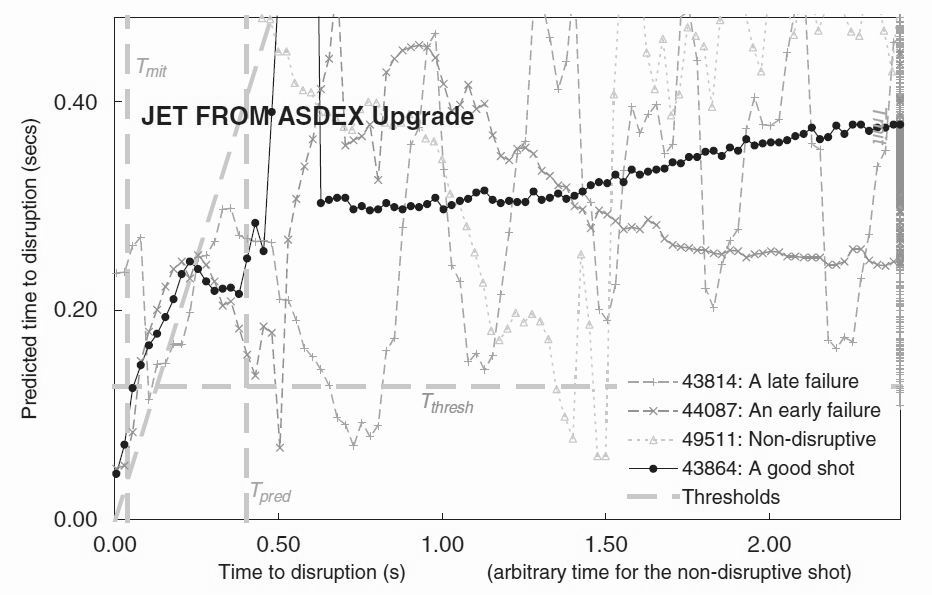
Figure 7. A version of figure 6(a) with the time axis extended by a factor of 5 and with only a selection of shots shown. The time origin of the non-disruptive shot is arbitrarily adjusted to fit in the centre of the page. With the same notation as in figure 2, a 'good' shot, 'early', 'late', and 'non-disruptive' failures are shown by full circles, triangles, crosses and feint triangles respectively. The example good shot is shown by black diamonds.

Figure 7 explores the approach to disruption over a longer time scale than the previous figures. The data and thresholds are identical. However the time scale has been increased by a factor 5 and only a selection of mostly failing shots is shown. The notation is similar to figure 2 except that a non-disruptive shot has been displayed on an arbitrary time axis.

A typical good prediction, say shot 43864, only achieves a reasonable agreement between predicted and actual time to disruption at times of order 0.3 sec. At greater times to disruption, the predicted time to disruption levels off at around 0.3 to 0.6 seconds. There is little information in the input parameters to suggest the presence of the oncoming disruption until 0.3 seconds or so before the disruption. This justifies our choice of training data, with its emphasis on times close to the disruption and its increasingly sparse information at longer times to disruption.

Of the two disruption prediction failures, shot 43814 shows an incipient disruption at around 0.8 seconds before the disruption. This is an ICRH heated pulse in which the coupling is repeatedly lost and re-established with the radiated power just before ICRH coupling is re-established rising close to the input power - a likely indicator of an imminent disruption. It is observed that the minima in the time to disruption corresponds well with peaks in radiated power and the ICRH coupling being re-established. These peaks end 0.8 seconds before the disruption, and the predicted time to disruption recovers well to give rather close agreement between predicted and actual times to disruption. However the predicted time to disruption suddenly rises to give a 'late' error. Shot 44087 follows a steady decrease in the predicted time to disruption around 0.7 to 0.5 seconds before the disruption. Once again it recovers but later follows a classic approach to the disruption.

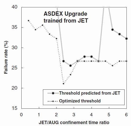
Figure 8. The corresponding plot to figure 5 showing the disruption prediction failure rate for ASDEX Upgrade data tested using a network trained on the JET data, as a function of the time ratio between JET and ASDEX Upgrade (average confinement times).

The non-disruptive shot 49511 is shown plotted against an arbitrarily shifted time, adjusted so that the interesting time region occurs in the centre of the figure. The actual scale is measured as if a disruption occurred at 21.56 seconds. The two dips below the threshold in the time to disruption therefore correspond to real times of 20.06 to 20.088 and 20.163 to 20.213 seconds. In fact from 19.85 to 20.00 seconds the NBI plasma heating was rapidly ramped down from 14 MW to zero. This may have got the plasma close to a radiative collapse (although the density remains well below the Greenwald limit). The bolometer exhibits two peaks after the NBI power was turned off, one at 20.03 seconds the other at 20.17 seconds with the bolometer power to total power ratio peaking at 8 then 3 MW, well exceeding the input power of around 1 MW at this time. In this sense the network is accurately reflecting that an unsustainable level of radiation is happening at this time. Although the plasma survived in this case, it is known that too rapid a switch off of heating power on JET can lead to disruption, and so the network was correctly indicating a high potential for disruption.

8. Results, training on JET and testing on ASDEX Upgrade

The situation is readily reversed so that ASDEX Upgrade data is tested on a network trained on JET data. It initially proved difficult to get good results for this case. Improved results (see figures 8 and 9) were obtained by addressing the normalisation (mapping them into the 0?1 range) of the parameters for Power Fraction, P5, and Normalised Confinement, P6. As Table 3 indicated these can be a factor of 2 or so larger for ASDEX Upgrade than for JET. However it must be emphasised that the left hand side of Table 3 refers only to the extreme values, rather than to more typical spreads. Typically on both tokamaks a few shots show up as 'outliers' with values exceeding the average spread in the data by 100% or more. Simple normalisation to the largest values was not a problem in the JET from ASDEX Upgrade predictions. However in the reverse direction, it is as if the detail in the JET test tokamak Normalised Confinement parameter has been "lost in the noise" (with little dynamic range in the JET data) when trained with the generally larger ASDEX Upgrade parameter. For the AUG trained network of section 7, normalising to the JET values greatly improved the JET prediction, but of course at the expense of a decreased performance for the ASDEX Upgrade single machine prediction performance.

The right hand side of Table 3 shows the lower and upper limits of the parameters when they are estimated from a histogram of the data against each parameter. Here the low value is when the histogram first exceeds 10% of the total area and the high value when the histogram last falls below 90% of the total area. These histogram limits give much more understandable ranges for the parameters. Sample studies show that these histogram limits lead to similar values to those reported in the paper.

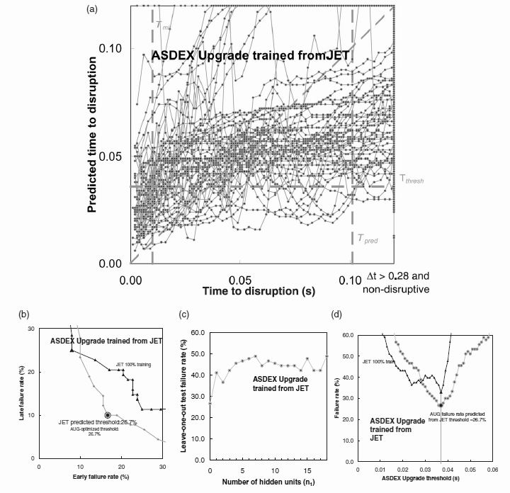
Figure 9. The corresponding plot from figure 6 corresponding to ASDEX Upgrade data tested using a network trained on the JET data. All variables have been included in this test. A simple perceptron with 100% learning has been used, except in the hidden unit plot of figure 9c.

Figure 8 shows that for a JET-trained network, the best predictive performance is obtained for a JET/AUG confinement time ratio of around 3, although a factor 4 still gives good performance. The best ASDEX Upgrade performance when the time factor and threshold are independently optimised in figure 8, is 26.7% achieved at a time ratio of 2.4. Figure 9a has many features similar to figure 6a. Again the predicted time to disruption is generally some 0.02 seconds longer than the actual time within 0.04 seconds of the disruption. At larger times before the disruption times we have a flattening off of the predicted time to disruption to a limit of around 0.06 seconds. It follows that the network has little cross-tokamak prediction capacity at times greater than 0.06 seconds before the disruption. The best prediction performance of 26.7 % (Fig 9b) is obtained including all the parameters but including any hidden units degrades performance (figure 9c). Table 2 shows that once again all feature parameters contribute positively to the prediction. Figure 9d shows that threshold times are again consistent between the devices, giving an optimal prediction for ASDEX Upgrade performance of 26.7% failure rate.

9. Conclusions

Neural network techniques previously used for predicting disruptions on a single tokamak have been extended to make cross machine predictions of disruption time on one tokamak, based on networks trained on another tokamak. This has been achieved by using a reduced set of dimensionless input parameters and simplified network structures that are better able to accommodate the degree of extrapolation required between tokamaks.

For a single tokamak (training and testing on the same tokamak), neural networks can predict disruptions with around 80 to 90% accuracy, even with a reduced input parameter set compared to previous studies. Optimum performance is obtained using multi-layer perceptrons with several hidden units. When predictions are made between tokamaks (JET and ASDEX Upgrade), an accuracy in the 70% range has been obtained, with optimum performance using a simple single layer perceptron.

Best results have been obtained with a target based on the time to disruption divided by an average confinement time for a given tokamak. In predicting performance on the second tokamak, an overall time scaling factor must be applied to all time-to-disruption and confinement time type measurement. This can be predicted from arguments based on resistive timescale for the disruption process, giving a factor 4 between AUG and JET, which is in close agreement with the empirically optimised time scale factor between tokamaks. This provides a "first principles" method of applying the data set to new devices without measurement of disruptive behaviour on those devices.

Further performance improvements are possible if threshold times for disruption prediction are allowed to vary independently of the above time factor between tokamaks. This also leads to optimum cross-machine performance for time factors significantly different from the above factor 4, but requires data from the test tokamak to determine the appropriate threshold level. With the cross-machine predictions, there is a danger of "over-learning" which is minimised by using the simple perceptron with no hidden units, and is found to give the best cross-machine performance. Care must also be taken with input parameter normalisation when the parameter ranges are different on the two tokamaks. Neural network input parameters are usually further normalised to fill a 0 to 1 input range. However with a degree of extrapolation between different tokamaks, the likely operating range of the test tokamak must be anticipated for reasonable performance to be maintained.

These studies are encouraging and indicate that the potential key weakness of the neural network approach to disruption prediction in a newly constructed tokamak, the need for a large training set of disruptions, might be overcome by training using data from a pre-existing tokamak (or tokamaks). This offers the basis of a potentially useful technique for large future devices such as ITER, to help reduce disruption frequency and avoid the need for a large disruption campaigns to train disruption avoidance systems. It would also enable that device to operate in a more cautious manner, until the safety of particular scenarios was established. Further work is needed to explore variations in performance and optimisation with key parameters such as T_mitTmit and T_pred (assumed from previous studies in this work). In addition, for a more cautious operational approach, more natural disruptions ("late failures" which here account for ~10-20% in the best networks) could be avoided, at the expense of an increased number of network-triggered terminations, which may be considered as safer more controlled events. The present failure rate of 30% may be too high to be acceptable and so although the results presented here are a positive step, further refinements are desirable. The technique described here could also be extended to disruptions in regimes other than the ELMy H-mode, or to include data from other tokamaks.

Acknowledgements

This work was conducted partly under the European Fusion Development Agreement and was funded in part the UK Engineering and Physical Sciences Research Council and by EURATOM. The authors acknowledge fruitful discussions with their many colleagues at Culham and Garching. The authors would like to thank their two referees for their valuable suggestions.

References

[1] Wesson J.A., Tokamaks, Clarendon Press, Oxford, 1987

[2] Wesson J.A. et al, "Disruptions in JET", Nuclear Fusion 29 (1989) 641-666.

[3] Tichmann Ch., Pautasso G., Fuchs J.C., Lackner, K., Mertens V.,, Morabito F.C., Schneider, W. and the ASDEX Upgrade Team. Use of a neural network for the prediction of disruptions in ASDEX Upgrade, 26th EPS conf. On Contr. Fusion and Plasma Physics, ECA Vol. 23J 761-764 1999.

[4] Wroblewski, D., Jahns, G.L. and Leuer, J.A., Nuclear Fusion 37, 725-741 1997.

[5] Milani F., "Disruption prediction at JET", Thesis: University of Aston at Birmingham, UK, 1998

[6]Yoshino R., "Neural-net disruption predictor in JT-60U", Nuclear Fusion, 43, 1771-1786, 2003

[7] Hernandez J.V., Vannucci A., Tajima T., Lin Z., Horton, W. and Mccool, S.C. "Neural Networks Prediction of some classes of tokamak disruptions", Nuclear Fusion, 36, 1009-1017,1996.

[8] Vannucci A., Oliveira K.A. and Tajima T., Forecast of TEXT plasma disruptions using soft X rays as input signal in a neural network", Nuclear Fusion, 39, 255-262,1999.

[9] Sengupta A. and Ranjan, P., Forecasting disruptions in the ADITYA tokamak using neural networks", Nuclear Fusion 40, 1993-2008, 2000.

[10] Bishop C.M, Neural networks for pattern recognition, Clarendon Press, Oxford, (1996)

[11] Pautasso G., Egorov S., Tichmann Ch., Fuchs J.C., Herrmann A., Maraschek M., Mast F., Mertens V., Percermeier I., Windsor C.G., Zehetbauer T. and the ASDEX Upgrade Team. Prediction and mitigation of disruptions in ASDEX Upgrade, Journal of Nuclear Materials 290-293, 1045-1051, 2001.

[12] Pautasso G., Tichmann C., Egorov S., Zehetbauer T., Gruber O., Maraschek M., Mast F., Mertens V., Percermeier I., Raupp, F., Treutterer, W., Windsor C.G., and the ASDEX Upgrade Team. On-line prediction and mitigation of disruptions in ASDEX Upgrade, Nuclear Fusion 42, (2002), 100-108.

[13] Franzen, P., Kaufmann, M., Mertens, V.F., Neu, G., Raupp, F., Zehetbauer, T. and the ASDEX Upgrade team, "On-line confinement regime identification for the discharge control system at ASDEX Upgrade", Fusion Technology, 33, 84-95, 1998

[14] Cannas B., Fanni, A., Marongiu E., and Sonato, P., "Disruption forecasting at JET using neural networks", Nuclear Fusion, 44, 68-76,2004.

[15] Parallel Distributed Processing, Ed. McClelland J and Rumelhart D E, MIT Press, 1987.

[16] Industrial Applications of Neural Networks: Project ANNIE Handbook, Mason, J P and Croall, I F, Springer Verlag, 1992.

[17] Introduction to Radial Basis Function Networks, Orr M.J.L., http://www.anc.ed.ac.uk/~mjo/intro/intro.html

 Copyright 2004: Colin Windsor: Last updated 17/6/2005